The Guts n’ Glory of Database InternalsB+Tree
The absolute worst thing about B+Trees is their name. It is like someone maliciously considered all the possible names and then selected the most confusing one.
A B+Tree is a very different animal from a binary tree, in particular. In the previous post, we looked at how we can implement a binary tree using raw file I/O. The problem here is that the cost of doing that is incredibly high. The cost of searching a binary tree is O(logN), which is considered good, but as it turns out, the actual cost of doing that with a file is really high. A seek time on a high end HDD is about 12ms(!) the seek time on a high end SSD is 0.15 ms (!!) *.
* If you ever wondered why pretty much every database vendor jumped on the SSD bandwagon, that kind of difference in performance is a very large part of it.
So, let us assume that we have 100 records in our database, log2(100) would be 7, on an HDD it will take ~ 84ms just to do seeks (and just over 1ms on SSD). Remember, this is when we have a mere hundred records. What happens if we have ten thousand? The log2(10000) would be 14 (13.28, actually, but we need to round up), which would cost us 168ms on HDD and over 2 ms on SSD.
Consider the fact that those data sizes don’t even count as toy databases, they are the stage where you throw everything into a file and do sequential scans over the whole dataset to find anything, because it is faster (dev time and what the user will feel) than any other solution.
So something must have been done about it, because databases larger than a million records exists with response time of under 1/4 of a second. And the answer to that is the B+Tree. Instead of tracking each value individually, we’ll define pages. A page is a fixed size, typically 4KB in size, that can contain a number of values. Instead of working with each individual values, we will work on pages. Let us consider the users example, and see how this works.
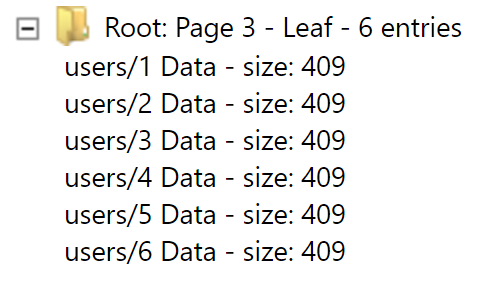
Now, all 3 entries are stored in the same page. And we store them sorted inside the page. Assuming a reasonable size of data per record, we can store multiple records in this single page. This allows us to take advantage on an interesting property of I/O, the costly thing is going to the hardware, less so how much work you do there. So the cost of reading 400 bytes or the cost of reading 4KB are basically the same*.
* This is actually a lie, on several levels. Reading 32KB or reading 64KB from disk has roughly the same performance. But reading 400 bytes and 4KB is exactly the same cost, because the OS will never issue a 100 bytes read, it will read 4KB at once, and then server the next reads from the cache (and frequently it will do read ahead, too).
Once we have the page in memory, we do a binary search inside the page to find that particular value. So for the records in the image above, the binary tree method would result in 3 disk accesses, and the page method will have just one. Clearly, the page method is better, but eventually you are going to run out of space in the page, what do you do then?
That is when you introduce a new level, and actually get a tree.
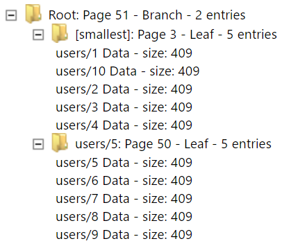
Now we have a much more interesting setup. We have two leaf pages, each of which holds the actual data for the users. And we have a branch (and root) page that holds the lowest key of the page that it points to. The logic for finding a particular value in this setup goes like this:
- Read the root page
- Do a binary search on the page to find the first key that is larger than the key you are searching for
- Load the previous key’s page.
- Search for the value in this page.
In other words, if we are searching for “users/4”, we first load the root page, and we find that users/5 is bigger than users/4. So we go to the previous one, which is Page 3. We load Page 1 and do a binary search there to find users/4. The name of the action that happens when the page is full and need more space is called a Page Spilt. In the case above, we had a page split at exactly users/10, which is a random write, as far as the B+Tree is concerned (we are doing lexical comparisons. Let us see how it would split in the case of sequential inserts.
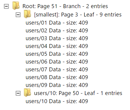
In this case, when we hit a page full we did it with a value that was supposed to go at the end of the page, so it is threated as a sequential insert, so instead of splitting the page, we can just allocate a new page, put the new value there, and then wire it to a parent. This allows us to avoid wasting space when we are doing sequential writes. Note that this particular behavior is a (pretty common) optimization in the implementation that I’m using.
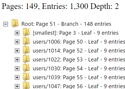
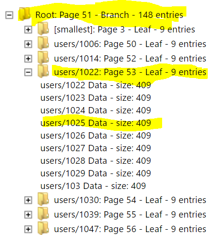
There are a few important things to remember here, the number of entries that can fit into a leaf page is primarily limited by the size of the values. In this case, in the pictures above, each value is exactly 409 bytes in size, and we can fit 9 of them into a single page. But the size of the branch page is the limited by the size of the key alone. So let us see what happens when we start writing a lot of new records. We wrote a total of 1,300 records, and we ended up with a root page that is has about 150 leaf pages.
If I want to find the record for users/1025, I need to first read the root page, and then do a binary search there. I find that the entry users/1030 is the first entry that is larger than it, so I go to page 54, and do a binary search there, finding the right value.
All I had to do was two disk operations. If I were using a binary tree, I would have to do 11 disk requests, and the performance difference would be 14 ms on a HDD for the B+Tree and 154 ms for the binary tree. Note that in terms of comparisons, I have to make 12 comparisons in the B+Tree, and 11 in the binary tree. I don’t count that time, since in memory work is effectively free in the context of any I/O work.
But our tree is now on a precarious situation, what would happen when we continue to add records to it? The root page is going to be full at some point, right? Here is what happens after we continue to add more items:
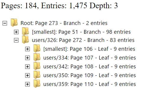
The depth of the tree has increased. We now have a depth of 3, and all queries will need 3 disk operations to complete. The cost has increased, but we are still an order of magnitude cheaper than the binary tree work.
Note that in this case, we have a total of 590 Kb of data, but the overhead is 736 Kb. This is because we can only fit 9 entries in a page, leaving us about 400 bytes unused. We also insert effectively random data, so we have page splits in the middle, which may have less records than that.
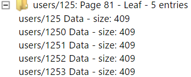
In this particular case, we’ve a total of 31 leaf pages with 5 entries (out of 176 leaf pages). So the total wasted space is about 50KB that are lost because of uneven page splits.
Note that a B+Tree with values of this size is extremely strange. Typically the size of an entry is in the a few tens of bytes (we’ll talk about larger values later), and a single page contains tens of records or more. If we consider 50 entries per page, then the same amount of pages will allow us to hold eight times more data. The key part, regardless of the number of records, is that this allows us to do so in very few disk accesses.
Notice that so far I didn’t really talk about balancing, which is a crucial part of how you deal with in memory trees. A B+Tree doesn’t need rebalancing all the time, but it does have a pretty crucial behavior when we reached the limit of a page. To make things simple, we’ll talk about a leaf page, but the same holds true for a branch page as well. Because the page is full, we need to split it. If your data is inserted in sequential manner, it is easy to see that we’ll only split when the a page is as full as it can be, and new inserts will go to new pages. It also means that we have the minimal possible depth of the tree, because the number of splits we have is so much lower.
On the other hand, in the case above we inserted 1,475 random entries, and created a non optimal B+Tree. It is important to observe that no optimal B+Tree doesn’t mean something catastrophic. In the case of keys like the one we see here, the data actually is going to become sorted (one we have enough digits in the number so it wouldn’t increase often), so it the issue will sort itself out, if you pardon the pun.
In the case of truly random data (guids, names, urls, etc), there is no real good way to have it sort out, and we just have to live with the tree fragmentation. This fragmentation leads to deeper trees, which means more disk seeks. That is why all databases really like it when you feed them sequential data. That is naturally the least work they have to do.
In practice, databases will do things like steal entries from nearby pages to ensure some balance, run cleanup procedures to see if they can trim the tree and in general try to fix this issue. The problem is that all of those behaviors are based of heuristics, and they can result in pretty bad performance. The good thing about fragmented tree is that once you reach a certain fragmentation level, you can usually add new data to the page (which is typically not full) without forcing additional splits. The bad part is that you are using more disk space and more disk operations. But sometimes that is the cost that you have to pay.
This post is getting long enough as it is, so I’ll continue the discussion on the usage of B+Trees in databases in my next post. In closing, I’ll note that the pretty pictures that you saw in the post are actually real output generated for a live RavenDB system. You can go to any Voron based database and ask it to print out its internal structure, and it will do as you command. The url to use is: http://[your-ravendb-server]/databases/[your-ravendb-database]/admin/voron/tree?name=documents
This is a debug level command, meant for us to inspect the internal state of the database, don’t use in production, etc.
More posts in "The Guts n’ Glory of Database Internals" series:
- (08 Aug 2016) Early lock release
- (05 Aug 2016) Merging transactions
- (03 Aug 2016) Log shipping and point in time recovery
- (02 Aug 2016) What goes inside the transaction journal
- (18 Jul 2016) What the disk can do for you
- (15 Jul 2016) The curse of old age…
- (14 Jul 2016) Backup, restore and the environment…
- (11 Jul 2016) The communication protocol
- (08 Jul 2016) The enemy of thy database is…
- (07 Jul 2016) Writing to a data file
- (06 Jul 2016) Getting durable, faster
- (01 Jul 2016) Durability in the real world
- (30 Jun 2016) Understanding durability with hard disks
- (29 Jun 2016) Managing concurrency
- (28 Jun 2016) Managing records
- (16 Jun 2016) Seeing the forest for the trees
- (14 Jun 2016) B+Tree
- (09 Jun 2016) The LSM option
- (08 Jun 2016) Searching information and file format
- (07 Jun 2016) Persisting information


Comments
What happens if lets say we have 2 branches both full and i need to insert a new record that has lower key than the lowest one i the second branch?
Luka,
That will cause a page split on the leaf, and then a page split on the parent branch, potentially page splitting all the way to the root
Wouldn't that lead to fragmentation?
Luka,
Yes, it would, but that is the nature of the beast when you are making non seuqntial inserts
Typo: "I find that the entry users/1030 is the first entry that is larger than it, so I go to page 54" should be "page 53"
Comment preview