Oren Eini

CEO of RavenDB

a NoSQL Open Source Document Database

Get in touch with me:

oren@ravendb.net +972 52-548-6969

Posts: 7,523
|
Comments: 51,145
Privacy Policy · Terms
filter by tags archive
time to read 5 min | 997 words

In my previous post, I showed how we use the nibble offload approach to store the size of entries in space that would otherwise be unused. My goal in that post was clarity, so I tried to make sure that the code was as nice to read as possible. In terms of machine code, that isn’t really ideal. Let’s talk about how we can make it better. Here is the starting version:

This code generates a function whose size exceeds 600 bytes and contains 24(!) branches. I already talked before about why this is a problem, there is a good discussion of the details on branches and their effect on performance here. In short, fewer branches are better. And when looking at machine instructions, the smaller the function, the better we are.

The first thing to do then is to remove the switch statement and move to a table-based approach. Given that this is a lookup of a small set of values, we can precompute all the options and just do a lookup like that. Here is what the code looks like:

This is already a win, since we are now at about half the code size (340 bytes) and there are just 7 branches in the function. Let’s take a look at the code and its assembly:

Code Assembly

if (inlined == 0)
{
     writeOffset = 1;
     buffer[0] = (byte)(keyLen << 4 | valLen);
}

L0065: test r14d, r14d
L0068: jne short L0081
L006a: mov r15d, 1
L0070: mov ecx, ebx
L0072: shl ecx, 4
L0075: or ecx, ebp
L0077: test edi, edi
L0079: je L014f
L007f: mov [rsi], cl

As you can see, in the assembly, we first test the value, and if it isn’t zero, we jump after the if statement. If it is 0, we compute a shift right by 4 and then or the values, then we do another check and finally set the value in the buffer.

Where does this check came from? There is no if there?

Well, that is the bound checking that we have with using Span, in fact, most of the checks there are because of Span or because of the safe intrinsics that are used.

Let’s get rid of this. There are actually several interesting iterations in the middle, but let’s jump directly to the final result I have. It’s under 10 lines of code, and it is quite beautiful.

I’m sure that you’ll look at this versus the previous iterations and go… huh?! I mean, even the reference table is different now.

Let’s analyze what is going on here in detail. The first thing you’ll note that changed is the method signature. Before we had multiple result types and now we use out parameters. This turns out to generate slightly less code, so I went with that approach, instead.

Next, computing the number of bytes we need to copy is the same. Once we have the sizes of the key and the value, we fetch the relevant instruction from the reference table. We do that in a way that skips the bounds checking on the table, since we know that we cannot exceed the length of the array.

Unlike before, we have new values in the table, where before we had 0 for entries that we didn’t care for, now we put 16. That means that we need to clear that when we set the nibble parameter. The reason for this is that we use this to compute the writeOffset. For cases where we have an offboarded nibble, the shift we do there will clear all the values, leaving us with a zero. For the values we cannot offload, we get 16, shifting by 4 gives us 1.

The reason we do it this way is that we do not use any conditional in this method. We unconditionally set the first byte of the buffer, because it is cheaper to do the work and discard that than check if it needs to be done.

Finally, we previously used Span.Copy() to move the data. That works, but it turns out that it is not ideal for very small writes, like what we have. At the same time, we write variable size each time, how can we manage that?

The answer is that we know that the buffer we are passed is large enough to contain the largest size possible. So we don’t need to worry about bound checking, etc.

We take advantage of the fact that the data is laid out in little-endian format and just write the whole 8 bytes of the key to the buffer at the right location. That may be shifted by the computed writeOffset. We then write the value immediately following the computed key length. The idea is that we overwrite the memory we just wrote (because parts of that were found to be not interesting). Using this approach, we were able to drop the code for this function to 114 bytes(!). Even with the encoding table, that is under three cache lines for the whole thing. That is really small.

There are also no conditionals or branches throughout the process. This is a piece of code that is ready and willing to be inlined anywhere. The amount of effort to understand what is going on here is balanced against how much this function can achieve in its lifetime.

For reference, here is the assembly of the encoding process:

The EncodingTable deserves a better explanation. I generated it using the following code:

In other words, I basically wrote out all the options and generated the appropriate value for each one of the options. I’m using the value of 16 here to be able to get to the right result using some bit shifts without any conditionals. So instead of doing many conditions, I replaced this with a (small) table lookup.

In my next post, I’m going to try to handle the same process for decoding.

time to read 8 min | 1459 words

Moving to nibble encoding gave us a measurable improvement in the density of the entries in the page.   The problem is that we pretty much run out of room to do so. We are currently using a byte per entry to hold the size of the entry (as two nibbles, of 4 bits each). You can’t really go lower than that.

Let’s review again what we know about the structure of the data, we have an 8KB page, with three sections, fixed size header and variable size offsets and entries array. Here is what this looks like:

image

This is called a slotted page design. The idea is that the offset array at the bottom of the page is maintaining the sort orders of the entries, and that we can write the entries from the top of the page. When we need to sort the entries, we just need to touch the offsets array (shown in yellow in the image).

Given that we are talking about size and density, we spent a lot of time trying to reduce the size of the entries, but can we do something with the header or the offsets? The header is just 4 bytes right now, two shorts that denote the location of the bottom and the top position in the page. Given that the page is 8KB in size, we have to use 16 bits integer to cover the range. For offsets, the situation is the same. We have to be able to point to the entry location on the page, and that means that we have to reach 8KB. So the offsets are actually 16 bits ints and take two bytes.

In other words, there is a hidden overhead of 2 bytes per entry that we didn’t even consider. In the case of our latest success, we were able to push 759 entries into the page, which means that we are actually using 18.5% of the page just to hold the offsets of the entries. That is 1.48 KB that is being used.

The problem is that we need to use this. We have to be able to point to an entry anywhere in the page, which means that we have to reach 0 .. 8192. The minimum size we can use is 16 bits or two bytes.

Or do we?

16 bits gives us a range of 0 .. 65,535, after all. That is far in excess of what we need. We could use a 64KB page, but there are other reasons to want to avoid that.

To cover 8KB, we only need 13 bits to cover the range we need, after all. For that matter, we can extend that bit by 25%. If we decide that an entry should be 2 bytes aligned, we can access the entire page in 12 bits.

That means that we have 4 whole free bits to play with. The first idea is to change the offsets array from 16 bits ints to 12 bits ints. That would save us 380 bytes at 759 entries per page. That is quite a lot. Unfortunately, working with bits in this manner would be super awkward. We are doing a lot of random access and moves while we are building the page. It is possible to do this using bits, but not fun.

So we can set things up so we have a nibble free to use. We just used nibbles to save on the cost of variable size ints, to great success.

However, we don’t need just a nibble, we need two of them. We need to store the size of the key and the value in bytes. Actually, we don’t need two nibbles. The size of the key and the value maxes at 8 bytes, after all. We can encode that in 3 bits. In other words, we need 6 bits to encode this information.

We only have 4 bits, however. It is a really nice idea, however, and I kept turning that in my head, trying to come up with all sorts of clever ways to figure out how we can push 64 values in 4 bits. The impact of that would be pretty amazing.

Eventually, I realized that it is fairly easy to prove, using math, that there is no way to do so. Faced with this failure, I realigned my thinking and found a solution. I don’t need to have a perfect answer, I can have a good one.

4 bits give me a range of 16 values (out of the possible 64). If I give up on trying to solve the whole problem, can I solve a meaningful part of it?

And I came up with the following idea. We can do a two-stage approach, we’ll map the most common 15 values of key and value sizes to those 4 bits. The last value will be a marker that you have to go and look elsewhere.

Using just the data in the offset, I’m able to figure out what the location of the entry in the page is as well as the size of the key and value for most cases. For the (hopefully rare) scenarios where that is not the case, we fall back to storing the size information as two nibbles preceding the entry data.

This is a pretty neat idea, even if I say so myself, and it has a good chance to allow us to save about 1 byte per entry in the common case. In fact, I tested that and about 90% of the cases in my test case are covered by the top 15 cases. That is a pretty good indication that I’m on the right track.

All of that said, let’s look at how this looks in code:

I’m using a switch expression here for readability, so it is clear what is going on. If the key and value sizes are in one of the known patterns, we can put that in the nibble we’ll return. If the value is not, we’ll write it to the entry buffer.

The Set method itself had to change in some subtle but crucial ways, let’s look at it first, then I’ll discuss those changes:

As before, we encode the entry into a temporary buffer. Now, in addition to getting the length of the entry, we are also getting the nibble that we’ll need to store.

You can see the changes in how we work with the offsets array following that. When we need to update an existing value, we are using this construction to figure out the actual entry offset:

var actualEntryOffset = ((offsets[idx] & 0xFFF0) >> 3);

What exactly is going on here? Don’t try to figure it out yet, let’s see how we are writing the data:

top = (ushort)((top - reqEntryLen) & ~1); // align on two bytes boundary 

offsets[idx] = (ushort)(top << 3 | nibble);

Those two code snippets may look very odd, so let’s go over them in detail.

First, remember that we have an 8KB page to work with, but we need to use 4 bits for the size nibble we got from encoding the entry. To address the full 8,192 values in the page, we’ll need to reserve 13 bits. That is… a problem. We solve that by saying that the entry addresses must always be aligned on two bytes boundary. That is handled by clearing the first bit in the new top computation. Since we are growing down, that has the effect of ensuring aligned-by-two.

Then, we merge the top location and the nibble together. We know that the bottom-most of the top is cleared, so we can just move the value by 3 bits and we know that we’ve 4 cleared bits ready.

Conversely, when we want to read, we clear the first 4 bits and then we shift by three. That has the effect of returning us back to the original state.

A little bit confusing, but we managed to get to squeeze 784 entries into the page using the realistic dataset and 765 using the full one. That is another 3.5% of space savings over the previous nibble attempt and over 10% increase in capacity from the variable integer approach.

And at this point, I don’t believe that there is anything more that I can do to reduce the size in a significant manner without having a negative impact elsewhere.

We are not done yet, however. We are done with the size aspect, but we also have much to do in terms of performance and optimizations for runtime.

In the meantime, you can see my full code here. In the next post, we are going to start talking about the actual machine code and how we can optimize it.

time to read 4 min | 750 words

In my last post we implemented variable-sized encoding to be able to pack even more data into the page. We were able to achieve 40% better density because of that. This is pretty awesome, but we would still like to do better. There are two disadvantages for variable size integers:

  • They may take more space than the actual raw numbers.
  • The number of branches is high, and non-predictable.

Given that we need to encode the key and value together, let’s see if we can do better. We know that both the key and the value are 8 bytes long. Using little-endian systems, we can consider the number as a byte array.

Consider this number: 139,713,513,353 which is composed of the following bytes: [137, 7, 147, 135, 32, 0, 0, 0]. This is how it looks in memory. This means, that we only need the first 5 bytes, not the last 3 zero ones.

It turns out that there is a very simple way to compute the number of used bytes, like so:

This translates into the following assembly:

Which is about as tight as you can want it to be.

Of course, there is a problem. In order to read the value back, we need to store the number of bytes we used somewhere. For variable-sized integers, they use the top bit until they run out. But we cannot do that here.

Remember however, that we encode two numbers here. And the length of the number is 8 bytes. In binary, that means that we need 4 bits to encode the length of each number. This means that if we’ll take an additional byte, we can fit the length of both numbers into a single byte.

The length of the key and the value would each fit on a nibble inside that byte. Here is what the encoding step looks like now:

And in assembly:

Note that there are no branches at all here. Which I’m really stoked about. As for decoding, we just have to go the other way around:

No branches, and really predictable code.

That is all great, but what about the sizes? We are always taking 4 additional bits per number. So it is actually a single additional byte for each entry we encode. By using varint, the memory we encode numbers that are beyond the 2GB range, we’re already winning. Encoding (3,221,241,856), for example, will cost us 5 bytes (since we limit the range of each byte to 7 bits). The key advantage in our case is that if we have any case where either key or value needs to take an additional byte, we are at parity with the nibble method. If both of them need that, we are winning, since the nibble method will use a single additional byte and the variable size integer will take two (one for each number).

Now that we understand encoding and decoding, the rest of the code is basically the same. We just changed the internal format of the entry, nothing about the rest of the code changes.

And the results?

For the realistic dataset, we can fit 759 entries versus 712 for the variable integer model.

For the full dataset, we can fit 752 entries versus 710 for the variable integer model.

That is a 7% improvement in size, but it also comes with a really important benefit. Fewer branches.

This is the sort of code that runs billions of times a second. Reducing its latency has a profound impact on overall performance. One of the things that we pay attention to in high-performance code is the number of branches, because we are using super scalar CPUs, multiple instructions may execute in parallel at the chip level. A branch may cause us to stall (we have to wait until the result is known before we can execute the next instruction), so the processor will try to predict what the result of the branch would be. If this is a highly predictable branch (an error code that is almost never taken, for example), there is very little cost to that.

The variable integer code, on the other hand, is nothing but branches, and as far as the CPU is concerned, there is no way to actually predict what the result will be, so it has to wait. Branchless or well-predicted code is a key aspect of high-performance code. And this approach can have a big impact.

As a reminder, we started at 511 items, and we are now at 759. The question is, can we do more?

I’ll talk about it in the next post…

time to read 6 min | 1095 words

In my previous post, we stored keys and values as raw numbers inside the 8KB page. That was simple, but wasteful. For many scenarios, we are never going to need to utilize the full 8 bytes range for a long. Most numbers are far smaller.

In the example I gave in the last post, we are storing the following range of numbers (file offsets, basically). I’m using two test scenarios, one where I’m testing the full range (for correctness) and one where I’m testing files under 512 GB in size. Given that we are trying to compress the space, once we hit the 512GB mark, it is probably less urgent, after all.

Here are the number generations that I’m using:


What this means is:

Full data set Realistic data set
  •   3% in the first 128 bytes
  •   7% in the first 64 KB
  • 25% in the first 8 MB
  • 35% in the first 2 GB
  • 15% in the first 512 GB
  • 5% in the first 128 TB
  • 3% in the first 32 Petabytes
  • 2% in the first 4 Exabytes
  •   1% in the first 128 bytes
  •   2% in the first 64 KB
  • 27% in the first 8 MB
  • 35% in the first 2 GB
  • 25% in the first 512 GB


This is meant to verify that we can handle any scenario, in practice, we can usually focus on the first 512 GB, which is far more common.

Using both approaches, I can fit using my previous approach, up to 511 entries per page. That makes sense, we are storing the data raw, so how can we do better? Most of the time, we don’t need anywhere near 8 bytes per value. For that reason, we have variable length encoding, which has many names, such as variable size int, 7 bits integers, etc. I adapted some methods from the .NET codebase to allow me to operate on Spans, like so:

Let’s check what sort of savings we can get using this approach:

  • Under 127 bytes– 1 byte
  • 128 bytes .. 32 KB – 2 bytes
  • 32KB .. 8MB – 3 bytes
  • 8MB .. 2GB – 4 bytes
  • 2 GB .. 512 GB – 5 bytes
  • 512GB .. 128 TB – 6 bytes
  • 128TB .. 32 Petabytes – 7 bytes
  • 32 Petabytes .. 8 Exabytes – 8 bytes
  • Greater than 8 Exabytes – 9 bytes

That is really cool, since for the realistic data set, we can pack a lot more data into the page.

It comes with a serious issue, however. The data is no longer fixed size (well, that is the point, no?). Why is that a problem? Because we want to be able to do a binary search on that, which means that we need to be able to access the data by index. As usual, the solution is to utilize indirection. We’ll dedicate the bottom of the page to an array of fixed-size int (16 bits – sufficient to cover the 8KB range of the page) that will point to the actual location of the entry. Like before, we are going to reserve the first few bytes as a header, in this case we’ll use 4 bytes, divided into two shorts. Those will keep track of the writes to the bottom and the top of the page.

At the bottom, we’ll have the actual offsets that point to the entries, and at the top, we write the actual entries. Here is what this looks like:

Let’s see how our reading from the page will look now. As you can see, it is very similar to what we had before, but instead of going directly to the key by its offset, we have to use the indirection:

The offsets array contains the location of the entry in the page, and that is laid out as the [varint-key][varint-val]. So we read (and discard) the key from the offset we found (we have to do that to discover its size) and then we read and return the actual value.

Let’s look at how we implemented the actual binary search in the page:

This is a bog standard binary search, with the only interesting bit that we are going through the offsets array to find the actual location of the key, which we then read using variable size decoding.

The interesting part of this model happens when we need to set a value. Here is what this looks like, with my notes following the code.

This is quite a lot, I’ll admit. Let’s try to break up into individual pieces what is going on here.

First, we get the header values (bottom, top) and initialize them if empty (note that bottom is set to 4, after the header, while top is set to the end of the buffer). The idea is that the bottom grows up and the top grows down. This is called Slotted Page design and it is a staple of database design.

We then encode the key and the value into a temporary buffer. We need to do that so we’ll know what size the entry will take. Then we need to figure out if we are updating an existing record or creating a new one.

Updating an existing record is complex. This is because the size of the new record may be greater than the size of the old one. So we can’t put it in the same location. I’m handling this by just allocating new space for this entry, ignoring the old space that was allocated to it.

I’m not handling any deletes / space reclamation on this series. That is a separate subject, not complex, but fairly tedious to do properly. So I’m going to focus solely on writes.

Updates to an existing entry that also change its size aren’t in my test dataset, so I’m not worried about it too much here. I mention this to point out that variable length records bring with them considerations that we wouldn’t have run into with the fixed-size model.

And after all of this work? What are the results?

With the fixed-size version, we could fit 511 entries into the page. With the variable size int, however, we can do better.

For the realistic dataset, I can fit 712 entries for the page, and for the full dataset, 710 (there are very few very big elements even there, but we can see that it has an impact).

511 vs. 712 may not sound like much, but that is 40% increase in the number of entries that I can fit. To give some context, using 8KB pages, that is a difference of 5 MB per million entries. That adds up.

The question is, can we do better? More on that in my next post…

time to read 4 min | 749 words

I write databases for a living, which means that I’m thinking a lot about persistence. Here is a fun challenge that we went through recently. We have the need to store a list of keys and values and then lookup a value by key. Pretty standard stuff. The keys and values are both 64 bits integers. In other words, what I would like to have is:

Dictionary<long,long> lookup;

That would be perfect, except that I’ve to persist the data, which means that I have to work with raw bytes. It’s easiest to think about it if we have some code in front of us. Here is the interface that I need to implement:

As you can see, we have a byte buffer (8KB in size) and we want to add or lookup values from the buffer. All the data resides in the buffer, nothing is external. And we cannot unpack it in memory, because this is used for lookups, so this needs to be really fast.

The keys we are storing are file offsets, so they correlate quite nicely to the overall size of the file. Meaning that you’ll have a lot of small values, but also large ones. Given a key, we need to be able to look its value quickly, since we may run this lookup billions of times.

Given that I have 8KB of data, I can do the following, just treat the buffer as a sorted array, which means that I get a pretty easy way to search for a particular value and a simple way to actually store things.

Theoretically, given an 8KB page, and 16 bytes per each (key, value) entry, we can store up to 512 entries per page. But it turns out that this is just a theory. We also need to keep track of the number of items that we have, and that takes some space. Just a couple of bytes, but it means that we don’t have those bytes available. A page can now contain up to 511 entries, and even at full capacity, we have 14 bytes wasted (2 for the number of entries, and the rest are unused).

Here is what this looks like in code:

As you can see, we are creating two arrays, the keys are growing from the bottom of the page and the values are growing from the top. The idea is that I can utilize the BinarySearch() method to quickly find the index of a key (or where it ought) to go. From there, I can look at the corresponding values array to get the actual value. The fact that they are growing separately (and toward each other) means that I don’t need to move as much memory if I’m getting values out of order.

For now, I want to set up the playground in which we’ll operate. The type of data that you write into such a system is important. I decided to use the following code to generate the test set:

The idea is that we’ll generate a random set of numbers, in the given distribution. Most of the values are in the range of 8MB to 512GB, representing a pretty good scenario overall, I think.

And with that, we just need to figure out what metrics we want to use for this purpose. My goal is to push as many values as I can into the buffer, while maintaining the ability to get a value by its key as fast as possible.

The current approach, for example, does a binary search on a sorted array plus an extra lookup to the companion values array. You really can’t beat this, if you allow to store arbitrary keys. Here is my test bench:

This will insert key/value pairs into the page until it is full. Note that we allow duplicates (we’ll just update the value), so we need to keep track of the number of entries inserted, not just the number of insertions.  We also validate the structure at any step of the way, to ensure that we always get the right behavior.

This code runs as expected and we can put 511 values into the page before it gives up. This approach works, it is simple to reason about and has very few flaws. It is also quite wasteful in terms of information density. I would like to do better than 511 entries / pager. Is it possible to drop below 16 bytes per entry?

Give it some thought, I’m going to present several ways of doing just that in my next post…

time to read 3 min | 424 words

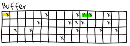
A few years ago I wrote about how you can use a bitmap to efficiently find space to allocate. I ran into a similar scenario recently and had another thought about that. Let’s say that we want to allocate from a buffer, which you can see below:

image

Set bits in the buffer (marked by X) are busy, and cleared bits are empty. We can find a range of cleared bits to allocate easily enough, as I have shown in my previous post.

The question we now need to answer is one of freeing the memory. In the image above, you can see that we have two allocations, the yellow one (the first item) and the green one (which is composed of two cells).

The problem is how do we know what to free in this case? In the case of yellow it is really easy since we can see that it is a single element. But freeing the green element is much harder since we can’t tell its size. Usually you need to keep that size somewhere, and usually you store it into the memory itself (taking some part of the allocation to yourself as metdata overhead).

The advantage of bitmaps is that they are simple, memory efficient, and quite fast. The problem is that they are really limited in what information they give us. The buffer above shows us busy or free, nothing more.

What if we’ll make it more interesting? Instead of using a single bit per cell, we’ll use two. Then we have the following states:

  • 0b00 – free
  • 0b11 – allocated (and has next)
  • 0b10 – end of allocation

This doubles the memory we use, but also gives us a really important property. Given an index in the bitmap, we can easily ask what the allocated is. We just need to find the next cleared bit, and compute the distance. Let’s consider this simple bitmap:

0b_00_01_00_01_11_11_00_01_11_01_01

As you can see, we have the following allocations (I separated each two bits to make it easy to show):

  • 0 – 1 cell
  • 1 – 1 cells
  • 2 – 2 cells
  • 5 – 3 cell
  • 9 – 1 cell

The code to do the actual accounting looks like this:

And now we have a bitmap where the cost of tracking the size of the allocation is a single additional bit.

If you are expecting a lot of big allocations, then this may not be worth it, but if you have many small allocations, removing the need to track this is a major benefit.

time to read 3 min | 555 words

We looked into the internal of Corax’s posting list and in the last post I mentioned that we have a problem with the Baseline of the page.

We are by no means the first people to work with posting lists, and there is a wide body of knowledge on the topic. When it came time to figure out the compression format for our posting list, we used the PFOR format (Patched Frame of Reference). It, like pretty much all other integer compression methods, uses 32 bits integers. Corax utilizes 64 bits integer as the document ids, so that was a problem. We solved that problem by using a Baseline for each page. In other words, each page would be able to contain values in a range of 2.1 billion of one another. That is a very reasonable range, given that a page is 8KB in size.

There was a problem as we built more features into Corax. The posting list needed to store not just the document id, but also the frequency of the term in the source document. It turns out that we need 8 bits to do so, and we already have 64 bits range so… Instead of creating another location to store the frequencies, we put them directly inside the posting list. But that meant that we reserved a range of bits. We have 64 bits overall, so not a big problem, right? Except that on a page basis, we have a lot less. Before, a page could contain a range of 2.1 billion, but we reserved 10 bits (frequency and tag, the details of which are not important to our story) and we ended up with a range that is 4 million per page. That little tidbit meant that we could only store in a page items that were within 4MB of one another. And that was a problem. Whenever we had a posting list where two values would be more than 4MB from one another, we would need to split the page. And since the posting list and the entries live on the same file, having more page splits means that entries are now further apart.

Here is an example of what this looks like:

image

The index is taking more space than the source data, and most of that is used to store… nothing, since we ended up with a very wide posting list containing very few entries. One of the cases of two independent issues compounding each other very quickly.

So we changed things again, instead of limiting ourselves to 32 bits range per page, we changed the PFor format to allow for 64 bits integers directly. Once again, that leads to simplification in the codebase and has greatly reduced the amount of disk space that we are actually using.

To give some context, here is the current amount of disk space taken by the same entity that previously took 800+GB:

image

The problem wasn’t with the number of entries, but that each entry would consume 8KB of disk space on its own, and in the image, you are seeing the number of posting lists, not the number of posting lists entries.

time to read 3 min | 594 words

In a previous post (which went out a long time ago) I explained that we have the notion of a set of uint64 values that are used for document IDs. We build a B+Tree with different behaviors for branch pages and leaf pages, allowing us to pack a lot of document IDs (thousands or more) per page.

The problem is that this structure hold the data compressed, so when we add or remove a value, we don’t know if it exists already or not. That is a problem, because while we are able to do any relevant fixups to skip duplicates and erase removed values, we end up in a position where the number of entries in the set is not accurate. That is a Problem, with a capital P, since we use that for query optimizations.

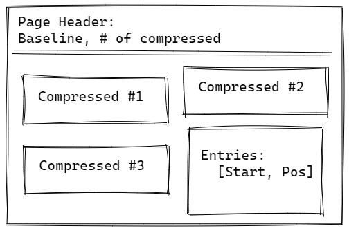
The solution for that is to move to a different manner of storing the data in the leaf page, instead of going with a model where we add the data directly to the page and compress when the raw values section overflows, we’ll use the following format instead:

image

Basically, I removed the raw values section from the design entirely. That means that whenever we want to add a new value, we need to find the relevant compressed segment inside the page and add to it (potentially creating a page split, etc).

Obviously, that is not going to perform well for write. Since on each addition, we’ll need to decompress the segment, add to it and then compress it again.

The idea here is that we don’t need to do that. Instead of trying to store the entries in the set immediately, we are going to keep them in memory for the duration of the transaction. Just before we commit the transaction, we are going to have two lists of document IDs to go through. One of added documents and one of removed documents. We can then sort those ids and then start walking over the list, find the relevant page for each section in the list, and merging it with the compressed values.

By moving the buffering stage from the per-page model to the per-transaction model, we actually gain quite a lot of performance, since if we have a lot of changes to a single page, we can handle compression of the data only once. It is a very strange manner of working, to be honest, because I’m used to doing the operation immediately. By delaying the cost to the end of the transaction, we are able to gain two major benefits. First, we have a big opportunity for batching and optimizing work on large datasets. Second, we have a single code path for this operation. It’s always: “Get a batch of changes and apply them as a unit”. It turns out that this is far easier to understand and work with. And that is for the writes portion of Corax.

Remember, however, that Corax is a search engine, so we expect a lot of reads. For reads, we can now stream the results directly from the compressed segments. Given that we can usually pack a lot of numbers into a segment, and that we don’t need to compare to the uncompressed portion, that ended up benefiting us significantly on the read side as well, surprisingly.

Of course, there is also another issue, look at the Baseline in the Page Header? We’ll discuss that in the next post, turned out that it wasn’t such a good idea.

time to read 3 min | 581 words

We care a lot about the performance of RavenDB, like a whole lot. To the point where we have a dedicated team that is continuously burning money CPU cycles testing out all sorts of scenarios with RavenDB. You can see the performance page on the website for some of their results. It got to the point where we stock NVMe drives at the office because we go through them often enough that we need them available for replacement. The benchmark must run, and the numbers must rise, after all.

But the story today isn’t about the costs we pay to reach our performance goals. Rather, it is about a curious little snafu that we ran into when looking at the results. Here are the benchmark results, I intentionally stripped out everything that will give context to this story. What you can see is the same scenario being run on two identical machines, with the difference being the disk that is being used to host the database.

image

In this case, the blue line is io1 disk (high IOPS, low latency, and high costs) versus gp3 (reasonable IOPS, much higher latency, and lower costs). In this case, lower numbers are better.

If you’ll look at the benchmark, you can see that it makes complete sense. RavenDB is a database product, we are running a benchmark, and we use the disk. It’s predictable that the disk latency will have an impact on the performance of the benchmark.

Except… in this case, we are looking at a benchmark that is read-only, and it is meant to run completely from memory. We wrote it so the data size is less than the amount of memory on the system. So why do we have an impact of the disk at all in this case?

We even have a warmup phase before we actually start measuring, to ensure that everything is in memory. Something here does not line up.

After investigating deeper, we discovered the following:

  • When running the automated benchmark, the performance was always correlated to the disk type.
  • When running the same benchmark, manually, there was much better performance and no slowdown related to the slower disk.

That is a really annoying bug, because the fact that we are observing it somehow makes it go away? What is going on?

After a while, we finally figured it out. The problem was the warmup phase. Basically, the warmup is just running the benchmark itself, discarding the results.

Can you guess what the problem was?

The warmup phase is running when the system is cold (naturally), we were hitting the server with enough requests up front that it was unable to process them all (it was queuing on the disk). That meant that a very large portion of the requests in the warmup would timeout or just fail. When we started the benchmark phase, significant portions of the system were still on the disk. So the benchmark become a disk-bound test, with predictable results.

When we ran it manually, we would always do that after the benchmark already run, so our system would be warm (and fast, with no disk access).

The solution for the problem was to scale down the number of requests that the warmup phase is running, to allow gradual loading of the data to memory, without overloading the hardware.

A case where our expectations and what really happened did not line up, creating some… interesting surprises in the end result.

FUTURE POSTS

No future posts left, oh my!

RECENT SERIES

  1. Challenge (75):
    01 Jul 2024 - Efficient snapshotable state
  2. Recording (14):
    19 Jun 2024 - Building a Database Engine in C# & .NET
  3. re (33):
    28 May 2024 - Secure Drop protocol
  4. Meta Blog (2):
    23 Jan 2024 - I'm a JS Developer now
  5. Production Postmortem (51):
    12 Dec 2023 - The Spawn of Denial of Service
View all series

Syndication

Main feed Feed Stats
Comments feed   Comments Feed Stats
}