Let’s say I want to count the number of reachable nodes for each node in the graph. I can do that using the following code:

void DFS(Node start, HashSet<Node> visited) 
{
    if (start == null || visited.Contains(start)) return;
    visited.Add(start);
    foreach (var neighbor in start.Neighbors) 
    {
        DFS(neighbor, visited);
    }
}


void MarkReachableCount(Graph g)
{
   foreach(var node in g.Nodes)
   {
       HashSet<Node> visited = [];
       DFS(node, visisted);
       node.ReachableGraph = visited.Count;
   }
}

A major performance cost for this sort of operation is the allocation cost. We allocate a separate hash set for each node in the graph, and then allocate whatever backing store is needed for it. If you have a big graph with many connections, that is expensive.

A simple fix for that would be to use:

void MarkReachableCount(Graph g)
{
   HashSet<Node> visited = [];
   foreach(var node in g.Nodes)
   {
       visited.Clear();
       DFS(node, visisted);
       node.ReachableGraph = visited.Count;
   }
}

This means that we have almost no allocations for the entire operation, yay!

This function also performs significantly worse than the previous one, even though it barely allocates. The reason for that? The call to Clear() is expensive. Take a look at the implementation - this method needs to zero out two arrays, and it will end up being as large as the node with the most reachable nodes. Let’s say we have a node that can access 10,000 nodes. That means that for each node, we’ll have to clear an array of about 14,000 items, as well as another array that is as big as the number of nodes we just visited.

No surprise that the allocating version was actually cheaper. We use the visited set for a short while, then discard it and get a new one. That means no expensive Clear() calls.

The question is, can we do better? Before I answer that, let’s try to go a bit deeper in this analysis. Some of the main costs in HashSet<Node> are the calls to GetHashCode() and Equals(). For that matter, let’s look at the cost of the Neighbors array on the Node.

Take a look at the following options:

public record Node1(List<Node> Neighbors);
public record Node2(List<int> NeighborIndexes);

Let’s assume each node has about 10 - 20 neighbors. What is the cost in memory for each option? Node1 uses references (pointers), and will take 256 bytes just for the Neighbors backing array (32-capacity array x 8 bytes). However, the Node2 version uses half of that memory.

This is an example of data-oriented design, and saving 50% of our memory costs is quite nice. HashSet<int> is also going to benefit quite nicely from JIT optimizations (no need to call GetHashCode(), etc. - everything is inlined).

We still have the problem of allocations vs. Clear(), though. Can we win?

Now that we have re-framed the problem using int indexes, there is a very obvious optimization opportunity: use a bit map (such as BitsArray). We know upfront how many items we have, right? So we can allocate a single array and set the corresponding bit to mark that a node (by its index) is visited.

That dramatically reduces the costs of tracking whether we visited a node or not, but it does not address the costs of clearing the bitmap.

Here is how you can handle this scenario cheaply:

public class Bitmap
{
    private ulong[] _data;
    private ushort[] _versions;
    private int _version;


    public Bitmap(int size)
    {
        _data = new ulong[(size + 63) / 64];
        _versions = new ushort[_data.Length];
    }


    public void Clear()
    {
        if(_version++ < ushort.MaxValue)
            return;
            
        Array.Clear(_data);
        Array.Clear(_versions);
    }


    public bool Add(int index)
    {
        int arrayIndex = index >> 6;
        if(_versions[arrayIndex] != _version)
        {
            _versions[arrayIndex] = _version;
            _data[arrayIndex] = 0;
        }


        int bitIndex = index & 63;
        ulong mask = 1UL << bitIndex;
        ulong old = _data[arrayIndex];
        _data[arrayIndex] |= mask;
        return (old & mask) == 0;
    }
}

The idea is pretty simple, in addition to the bitmap - we also have another array that marks the version of each 64-bit range. To clear the array, we increment the version. That would mean that when adding to the bitmap, we reset the underlying array element if it doesn’t match the current version. Once every 64K items, we’ll need to pay the cost of actually resetting the backing stores, but that ends up being very cheap overall (and worth the space savings to handle the overflow).

The code is tight, requires no allocations, and performs very quickly.

I ran into an interesting post, "Sharding Pgvector," in which PgDog (provider of scaling solutions for Postgres) discusses scaling pgvector indexes (HNSW and IVFFlat) across multiple machines to manage large-scale embeddings efficiently. This approach speeds up searches and improves recall by distributing vector data, addressing the limitations of fitting large indexes into memory on a single machine.

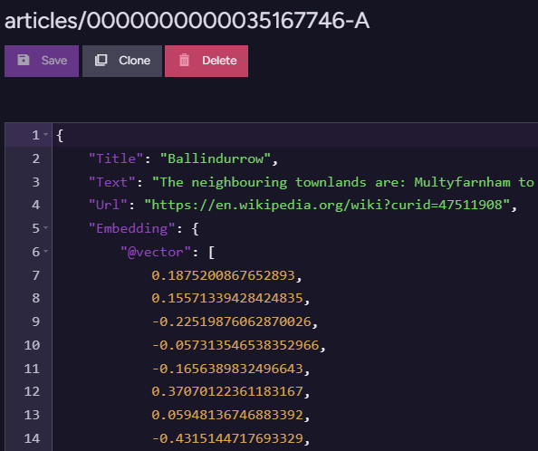
That was interesting to me because they specifically mention this Wikipedia dataset, consisting of 35.1 million vectors. That… is not really enough to justify sharding, in my eyes. The dataset is about 120GB of Parquet files, so I threw that into RavenDB using the following format:

Each vector has 768 dimensions in this dataset.

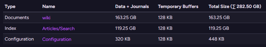
33 minutes later, I had the full dataset in RavenDB, taking 163 GB of storage space. The next step was to define a vector search index, like so:

from a in docs.Articles
select new 
{
    Vector = CreateVector(a.Embedding)
}

That index (using the HNSW algorithm) is all that is required to start doing proper vector searches in RavenDB.

Here is what this looks like - we have 163GB for the raw data, and the index itself is 119 GB.

RavenDB (and PgVector) actually need to store the vectors twice - once in the data itself and once in the index.

Given the size of the dataset, I used a machine with 192 GB of RAM to create the index. Note that this still means the total data size is about ⅓ bigger than the available memory, meaning we cannot compute it all in memory.

This deserves a proper explanation  - HNSW is a graph algorithm that assumes you can cheaply access any part of the graph during the indexing process. Indeed, this is effectively doing pure random reads on the entire dataset. You would generally run this on a machine with at least 192 GB of RAM.  I assume this is why pgvector required sharding for this dataset.

I decided to test it out on several different machines. The key aspect here is the size of memory, I’m ignoring CPU counts and type, they aren’t the bottleneck for this scenario. As a reminder, we are talking about a total data size that is close to 300 GB.

Note that all of those were run on a single machine, all using local NVMe disk. And yes, that is less than two days to index that much data on a machine that is grossly inadequate for it.

I should note that on the smaller machines, query times are typically ~5ms, so even with a lot of data indexed, the actual search doesn’t need to run on a machine with a lot of memory.

In short, I don’t see a reason why you would need to use sharding for that amount of data. It can comfortably fit inside a reasonably sized machine, with room to spare.

I should also note that the original post talks about using the IVFFlat algorithm instead of HNSW. Pgvector supports both, but RavenDB only uses HNSW. From a technical perspective, I would love to be able to use IVFFlat, since it is a much more traditional algorithm for databases.

You run k-means over your data to find the centroids (so you can split the data into reasonably sized chunks), and then just do an efficient linear search on that small chunk as needed. It fits much more nicely into the way databases typically work. However, it also has some significant drawbacks:

• You have to have the data upfront, you cannot build it incrementally.
• The effectiveness of the IVFFlat index degrades over time with inserts & deletes, because the original centroids are no longer as accurate.

Because of those reasons, we didn’t implement that. HNSW is a far more complex algorithm, both in terms of the actual approach and the number of hoops we had to go through to implement that efficiently, but as you can see, it is able to provide good results even on large datasets, can be built incrementally and doesn’t degrade over time.

Head-to-head comparison

I decided to run pgvector and RavenDB on the same dataset to get some concrete ideas about their performance. Because I didn’t feel like waiting for hours, I decided to use this dataset. It has 485,859 vectors and about 1.6 GB of data.

RavenDB indexed that in 1 minute and 17 seconds. My first attempt with pgvector took over 7 minutes when setting maintenance_work_mem = '512MB'. I had to increase it to 2GB to get more reasonable results (and then it was 1 minute and 49 seconds).

RavenDB is able to handle it a lot better when there isn’t enough memory to keep it all in RAM, while pgvector seems to degrade badly.

Summary

In short, I don’t think that you should need to go for sharding (and its associated complexity) for that amount of data. And I say that as someone whose database has native sharding capabilities.

For best performance, you should run large vector indexes on machines with plenty of RAM, but even without that, RavenDB does an okay job of keeping things ticking.

We recently tackled performance improvements for vector search in RavenDB. The core challenge was identifying performance bottlenecks. Details of specific changes are covered in a separate post. The post is already written, but will be published next week, here is the direct link to that.

In this post, I don’t want to talk about the actual changes we made, but the approach we took to figure out where the cost is.

Take a look at the following flame graph, showing where our code is spending the most time.

As you can see, almost the entire time is spent computing cosine similarity. That would be the best target for optimization, right?

I spent a bunch of time writing increasingly complicated ways to optimize the cosine similarity function. And it worked, I was able to reduce the cost by about 1.5%!

That is something that we would generally celebrate, but it was far from where we wanted to go. The problem was elsewhere, but we couldn’t see it in the profiler output because the cost was spread around too much.

Our first task was to restructure the code so we could actually see where the costs were. For instance, loading the vectors from disk was embedded within the algorithm. By extracting and isolating this process, we could accurately profile and measure its performance impact.

This restructuring also eliminated the "death by a thousand cuts" issue, making hotspots evident in profiling results. With clear targets identified, we can now focus optimization efforts effectively.

That major refactoring had two primary goals. The first was to actually extract the costs into highly visible locations, the second had to do with how you address them. Here is a small example that scans a social graph for friends, assuming the data is in a file.

def read_user_friends(file, user_id: int) -> List[int]:
    """Read friends for a single user ID starting at indexed offset."""
    pass # redacted


def social_graph(user_id: int, max_depth: int) -> Set[int]:
    if max_depth < 1:
        return set()
    
    all_friends = set() 
    visited = {user_id} 
    work_list = deque([(user_id, max_depth)])  
    
    with open("relations.dat", "rb") as file:
        while work_list:
            curr_id, depth = work_list.popleft()
            if depth <= 0:
                continue
                
            for friend_id in read_user_friends(file, curr_id):
                if friend_id not in visited:
                    all_friends.add(friend_id)
                    visited.add(friend_id)
                    work_list.append((friend_id, depth - 1))
    
    return all_friends

If you consider this code, you can likely see that there is an expensive part of it, reading from the file. But the way the code is structured, there isn’t really much that you can do about it. Let’s refactor the code a bit to expose the actual costs.

def social_graph(user_id: int, max_depth: int) -> Set[int]:
    if max_depth < 1:
        return set()
    
    all_friends = set() 
    visited = {user_id} 
    
    with open("relations.dat", "rb") as file:
        work_list =  read_user_friends(file, [user_id])
        while work_list and max_depth >= 0:
            to_scan = set()
            for friend_id in work_list: # gather all the items to read
                if friend_id in visited:
                    continue
                
                all_friends.add(friend_id)
                visited.add(friend_id)
                to_scan.add(curr_id)


            # read them all in one shot
            work_list = read_users_friends(file, to_scan)
            # reduce for next call
            max_depth = max_depth - 1    
    
    return all_friends

Now, instead of scattering the reads whenever we process an item, we gather them all and then send a list of items to read all at once. The costs are far clearer in this model, and more importantly, we have a chance to actually do something about it.

Optimizing a lot of calls to read_user_friends(file, user_id) is really hard, but optimizing read_users_friends(file, users) is a far simpler task. Note that the actual costs didn’t change because of this refactoring, but the ability to actually make the change is now far easier.

Going back to the flame graph above, the actual cost profile differs dramatically as the size of the data rose, even if the profiler output remained the same. Refactoring the code allowed us to see where the costs were and address them effectively.

Here is the end result as a flame graph. You can clearly see the preload section that takes a significant portion of the time. The key here is that the change allowed us to address this cost directly and in an optimal manner.

The end result for our benchmark was:

• Before: 3 minutes, 6 seconds
• After: 2 minutes, 4 seconds

So almost exactly ⅓ of the cost was removed because of the different approach we took, which is quite nice.

This technique, refactoring the code to make the costs obvious, is a really powerful one. Mostly because it is likely the first step to take anyway in many performance optimizations (batching, concurrency, etc.).

I recently reviewed a function that looked something like this:

public class WorkQueue<T>
{
    private readonly ConcurrentQueue<T> _embeddingsQueue = new();
    private long _approximateCount = 0;


    public long ApproximateCount => Interlocked.Read(ref _approximateCount);


    public void Register(IEnumerable<T> items)
    {
        foreach (var item in items)
        {
            _embeddingsQueue.Enqueue(item);


            Interlocked.Increment(ref _approximateCount);
        }
    }
}

I commented that we should move the Increment() operation outside of the loop because if two threads are calling Register() at the same time, we’ll have a lot of contention here.

The reply was that this was intentional since calling Interlocked.CompareExchange() to do the update in a batch manner is more complex. The issue was a lack of familiarity with the Interlocked.Add() function, which allows us to write the function as:

public void Register(IEnumerable<T> items)
{
    int count = 0;
    foreach (var item in items)
    {
        _embeddingsQueue.Enqueue(item);
        count++;
    }
    Interlocked.Add(ref _approximateCount, count);
}

This allows us to perform just one atomic operation on the count. In terms of assembly, we are going to have these two options:

lock inc qword ptr [rcx] ; Interlocked.Increment()
lock add [rbx], rcx      ; Interlocked.Add()

Both options have essentially the same exact performance characteristics, but if we need to register a large batch of items, the second option drastically reduces the contention.

In this case, we don’t actually care about having an accurate count as items are added, so there is no reason to avoid the optimization.

I care about the performance of RavenDB. Enough that I would go to epic lengths to fix them. Here I use “epic” both in terms of the Agile meaning of multi-month journeys and the actual amount of work required. See my recent posts about RavenDB 7.1 I/O work.

There hasn’t been a single release in the past 15 years that didn’t improve the performance of RavenDB in some way. We have an entire team whose sole task is to find bottlenecks and fix them, to the point where assembly language is a high-level concept at times (yes, we design some pieces of RavenDB with CPU microcode for performance).

When we ran into this issue, I was… quite surprised, to say the least. The problem was that whenever we serialized a document in RavenDB, we would compile some LINQ expressions.

That is expensive, and utterly wasteful. That is the sort of thing that we should never do, especially since there was no actual need for it.

Here is the essence of this fix:

We ran a performance test on the before & after versions, just to know what kind of performance we left on the table.

The fixed version is 1,689 times faster, if you can believe that.

So here is a fix that is both great to have and quite annoying. We focused so much effort on optimizing the server, and yet we missed something that obvious? How can that be?

Well, the answer is that this isn’t an actual benchmark. The problem is that this code is invoked per instance created instead of globally, and it is created once per thread. In any situation where the number of threads is more or less fixed (most production scenarios, where you’ll be using a thread pool, as well as in most benchmarks), you are never going to see this problem.

It is when you have threads dying and being created (such as when you handle spikes) that you’ll run into this issue. Make no mistake, it is an actual issue. When your load spikes, the thread pool will issue new threads, and they will consume a lot of CPU initially for absolutely no reason.

In short, we managed to miss this entirely (the code dates to 2017!) for a long time. It never appeared in any benchmark. The fix itself is trivial, of course, and we are unlikely to be able to show any real benefits from it in a benchmark, but that is yet another step in making RavenDB better.

One of the more interesting developments in terms of kernel API surface is the IO Ring. On Linux, it is called IO Uring and Windows has copied it shortly afterward. The idea started as a way to batch multiple IO operations at once but has evolved into a generic mechanism to make system calls more cheaply. On Linux, a large portion of the kernel features is exposed as part of the IO Uring API, while Windows exposes a far less rich API (basically, just reading and writing).

The reason this matters is that you can use IO Ring to reduce the cost of making system calls, using both batching and asynchronous programming. As such, most new database engines have jumped on that sweet nectar of better performance results.

As part of the overall re-architecture of how Voron manages writes, we have done the same. I/O for Voron is typically composed of writes to the journals and to the data file, so that makes it a really good fit, sort of.

An ironic aspect of IO Uring is that despite it being an asynchronous mechanism, it is inherently single-threaded. There are good reasons for that, of course, but that means that if you want to use the IO Ring API in a multi-threaded environment, you need to take that into account.

A common way to handle that is to use an event-driven system, where all the actual calls are generated from a single “event loop” thread or similar. This is how the Node.js API works, and how .NET itself manages IO for sockets (there is a single thread that listens to socket events by default).

The whole point of IO Ring is that you can submit multiple operations for the kernel to run in as optimal a manner as possible. Here is one such case to consider, this is the part of the code where we write the modified pages to the data file:

using (fileHandle)
{
    for (int i = 0; i < pages.Length; i++)
    {
        int numberOfPages = pages[i].GetNumberOfPages();


        var size = numberOfPages * Constants.Storage.PageSize;
        var offset = pages[i].PageNumber * Constants.Storage.PageSize;
        var span = new Span<byte>(pages[i].Pointer, size);
        RandomAccess.Write(fileHandle, span, offset);


        written += numberOfPages * Constants.Storage.PageSize;
    }
}

PID     LWP TTY          TIME CMD
  22334   22345 pts/0    00:00:00 iou-wrk-22343
  22334   22346 pts/0    00:00:00 iou-wrk-22343
  22334   22347 pts/0    00:00:00 iou-wrk-22334
  22334   22348 pts/0    00:00:00 iou-wrk-22334
  22334   22349 pts/0    00:00:00 iou-wrk-22334
  22334   22350 pts/0    00:00:00 iou-wrk-22334
  22334   22351 pts/0    00:00:00 iou-wrk-22334
  22334   22352 pts/0    00:00:00 iou-wrk-22334
  22334   22353 pts/0    00:00:00 iou-wrk-22334
  22334   22354 pts/0    00:00:00 iou-wrk-22334
  22334   22355 pts/0    00:00:00 iou-wrk-22334
  22334   22356 pts/0    00:00:00 iou-wrk-22334
  22334   22357 pts/0    00:00:00 iou-wrk-22334
  22334   22358 pts/0    00:00:00 iou-wrk-22334

Actually, those aren’t threads in the normal sense. Those are kernel tasks, generated by the IO Ring at the kernel level directly. It turns out that internally, IO Ring may spawn worker threads to do the async work at the kernel level. When we had a separate IO Ring per file, each one of them had its own pool of threads to do the work.

The way it usually works is really interesting. The IO Ring will attempt to complete the operation in a synchronous manner. For example, if you are writing to a file and doing buffered writes, we can just copy the buffer to the page pool and move on, no actual I/O took place. So the IO Ring will run through that directly in a synchronous manner.

However, if your operation requires actual blocking, it will be sent to a worker queue to actually execute it in the background. This is one way that the IO Ring is able to complete many operations so much more efficiently than the alternatives.

In our scenario, we have a pretty simple setup, we want to write to the file, making fully buffered writes. At the very least, being able to push all the writes to the OS in one shot (versus many separate system calls) is going to reduce our overhead. More interesting, however, is that eventually, the OS will want to start writing to the disk, so if we write a lot of data, some of the requests will be blocked. At that point, the IO Ring will switch them to a worker thread and continue executing.

The problem we had was that when we had a separate IO Ring per data file and put a lot of load on the system, we started seeing contention between the worker threads across all the files. Basically, each ring had its own separate pool, so there was a lot of work for each pool but no sharing.

If the IO Ring is single-threaded, but many separate threads lead to wasted resources, what can we do? The answer is simple, we’ll use a single global IO Ring and manage the threading concerns directly.

Here is the setup code for that (I removed all error handling to make it clearer):

void *do_ring_work(void *arg)
{
  int rc;
  if (g_cfg.low_priority_io)
  {
    syscall(SYS_ioprio_set, IOPRIO_WHO_PROCESS, 0, 
        IOPRIO_PRIO_VALUE(IOPRIO_CLASS_BE, 7));
  }
  pthread_setname_np(pthread_self(), "Rvn.Ring.Wrkr");
  struct io_uring *ring = &g_worker.ring;
  struct workitem *work = NULL;
  while (true)
  {
    do
    {
      // wait for any writes on the eventfd 
      // completion on the ring (associated with the eventfd)
      eventfd_t v;
      rc = read(g_worker.eventfd, &v, sizeof(eventfd_t));
    } while (rc < 0 && errno == EINTR);
    
    bool has_work = true;
    while (has_work)
    {
      int must_wait = 0;
      has_work = false;
      if (!work) 
      {
        // we may have _previous_ work to run through
        work = atomic_exchange(&g_worker.head, 0);
      }
      while (work)
      {
        has_work = true;


        struct io_uring_sqe *sqe = io_uring_get_sqe(ring);
        if (sqe == NULL)
        {
          must_wait = 1;
          goto sumbit_and_wait; // will retry
        }
        io_uring_sqe_set_data(sqe, work);
        switch (work->type)
        {
        case workitem_fsync:
          io_uring_prep_fsync(sqe, work->filefd, IORING_FSYNC_DATASYNC);
          break;
        case workitem_write:
          io_uring_prep_writev(sqe, work->filefd, work->op.write.iovecs,
                               work->op.write.iovecs_count, work->offset);
          break;
        default:
          break;
        }
        work = work->next;
      }
    sumbit_and_wait:
      rc = must_wait ? 
        io_uring_submit_and_wait(ring, must_wait) : 
        io_uring_submit(ring);
      struct io_uring_cqe *cqe;
      uint32_t head = 0;
      uint32_t i = 0;


      io_uring_for_each_cqe(ring, head, cqe)
      {
        i++;
        // force another run of the inner loop, 
        // to ensure that we call io_uring_submit again
        has_work = true; 
        struct workitem *cur = io_uring_cqe_get_data(cqe);
        if (!cur)
        {
          // can be null if it is:
          // *  a notification about eventfd write
          continue;
        }
        switch (cur->type)
        {
        case workitem_fsync:
          notify_work_completed(ring, cur);
          break;
        case workitem_write:
          if (/* partial write */)
          {
            // queue again
            continue;
          }
          notify_work_completed(ring, cur);
          break;
        }
      }
      io_uring_cq_advance(ring, i);
    }
  }
  return 0;
}

What does this code do?

We start by checking if we want to use lower-priority I/O, this is because we don’t actually care how long those operations take. The purpose of writing the data to the disk is that it will reach it eventually. RavenDB has two types of writes:

• Journal writes (durable update to the write-ahead log, required to complete a transaction).
• Data flush / Data sync (background updates to the data file, currently buffered in memory, no user is waiting for that)

As such, we are fine with explicitly prioritizing the journal writes (which users are waiting for) in favor of all other operations.

What is this C code? I thought RavenDB was written in C#

RavenDB is written in C#, but for very low-level system details, we found that it is far easier to write a Platform Abstraction Layer to hide system-specific concerns from the rest of the code. That way, we can simply submit the data to write and have the abstraction layer take care of all of that for us. This also ensures that we amortize the cost of PInvoke calls across many operations by submitting a big batch to the C code at once.

After setting the IO priority, we start reading from what is effectively a thread-safe queue. We wait for eventfd() to signal that there is work to do, and then we grab the head of the queue and start running.

The idea is that we fetch items from the queue, then we write those operations to the IO Ring as fast as we can manage. The IO Ring size is limited, however. So we need to handle the case where we have more work for the IO Ring than it can accept. When that happens, we will go to the submit_and_wait label and wait for something to complete.

Note that there is some logic there to handle what is going on when the IO Ring is full. We submit all the work in the ring, wait for an operation to complete, and in the next run, we’ll continue processing from where we left off.

The rest of the code is processing the completed operations and reporting the result back to their origin. This is done using the following function, which I find absolutely hilarious:

int32_t rvn_write_io_ring(
    void *handle,
    struct page_to_write *buffers,
    int32_t count,
    int32_t *detailed_error_code)
{
    int32_t rc = SUCCESS;
    struct handle *handle_ptr = handle;
    if (count == 0)
        return SUCCESS;


    if (pthread_mutex_lock(&handle_ptr->global_state->writes_arena.lock))
    {
        *detailed_error_code = errno;
        return FAIL_MUTEX_LOCK;
    }
    size_t max_req_size = (size_t)count * 
                      (sizeof(struct iovec) + sizeof(struct workitem));
    if (handle_ptr->global_state->writes_arena.arena_size < max_req_size)
    {
        // allocate arena space
    }
    void *buf = handle_ptr->global_state->writes_arena.arena;
    struct workitem *prev = NULL;
    int eventfd = handle_ptr->global_state->writes_arena.eventfd;
    for (int32_t curIdx = 0; curIdx < count; curIdx++)
    {
        int64_t offset = buffers[curIdx].page_num * VORON_PAGE_SIZE;
        int64_t size = (int64_t)buffers[curIdx].count_of_pages *
                       VORON_PAGE_SIZE;
        int64_t after = offset + size;


        struct workitem *work = buf;
        *work = (struct workitem){
            .op.write.iovecs_count = 1,
            .op.write.iovecs = buf + sizeof(struct workitem),
            .completed = 0,
            .type = workitem_write,
            .filefd = handle_ptr->file_fd,
            .offset = offset,
            .errored = false,
            .result = 0,
            .prev = prev,
            .notifyfd = eventfd,
        };
        prev = work;
        work->op.write.iovecs[0] = (struct iovec){
            .iov_len = size, 
            .iov_base = buffers[curIdx].ptr
        };
        buf += sizeof(struct workitem) + sizeof(struct iovec);


        for (size_t nextIndex = curIdx + 1; 
            nextIndex < count && work->op.write.iovecs_count < IOV_MAX; 
            nextIndex++)
        {
            int64_t dest = buffers[nextIndex].page_num * VORON_PAGE_SIZE;
            if (after != dest)
                break;


            size = (int64_t)buffers[nextIndex].count_of_pages *
                              VORON_PAGE_SIZE;
            after = dest + size;
            work->op.write.iovecs[work->op.write.iovecs_count++] = 
                (struct iovec){
                .iov_base = buffers[nextIndex].ptr,
                .iov_len = size,
            };
            curIdx++;
            buf += sizeof(struct iovec);
        }
        queue_work(work);
    }
    rc = wait_for_work_completion(handle_ptr, prev, eventfd, 
detailed_error_code);
    pthread_mutex_unlock(&handle_ptr->global_state->writes_arena.lock)
    return rc;
}

Remember that when we submit writes to the data file, we must wait until they are all done. The async nature of IO Ring is meant to help us push the writes to the OS as soon as possible, as well as push writes to multiple separate files at once. For that reason, we use anothereventfd() to wait (as the submitter) for the IO Ring to complete the operation. I love the code above because it is actually using the IO Ring itself to do the work we need to do here, saving us an actual system call in most cases.

Here is how we submit the work to the worker thread:

void queue_work(struct workitem *work)
{
    struct workitem *head = atomic_load(&g_worker.head);
    do
    {
        work->next = head;
    } while (!atomic_compare_exchange_weak(&g_worker.head, &head, work));
}

This function handles the submission of a set of pages to write to a file. Note that we protect against concurrent work on the same file. That isn’t actually needed since the caller code already handles that, but an uncontended lock is cheap, and it means that I don’t need to think about concurrency or worry about changes in the caller code in the future.

We ensure that we have sufficient buffer space, and then we create a work item. A work item is a single write to the file at a given location. However, we are using vectored writes, so we’ll merge writes to the consecutive pages into a single write operation. That is the purpose of the huge for loop in the code. The pages arrive already sorted, so we just need to do a single scan & merge for this.

Pay attention to the fact that the struct workitem actually belongs to two different linked lists. We have the next pointer, which is used to send work to the worker thread, and the prev pointer, which is used to iterate over the entire set of operations we submitted on completion (we’ll cover this in a bit).

Queuing work is done using the following method:

int32_t
wait_for_work_completion(struct handle *handle_ptr, 
    struct workitem *prev, 
    int eventfd, 
    int32_t *detailed_error_code)
{
    // wake worker thread
    eventfd_write(g_worker.eventfd, 1);
    
    bool all_done = false;
    while (!all_done)
    {
        all_done = true;
        *detailed_error_code = 0;


        eventfd_t v;
        int rc = read(eventfd, &v, sizeof(eventfd_t));
        struct workitem *work = prev;
        while (work)
        {
            all_done &= atomic_load(&work->completed);
            work = work->prev;
        }
    }
    return SUCCESS;
}

The idea is pretty simple. We first wake the worker thread by writing to its eventfd(), and then we wait on our own eventfd() for the worker to signal us that (at least some) of the work is done.

Note that we handle the submission of multiple work items by iterating over them in reverse order, using the prev pointer. Only when all the work is done can we return to our caller.

The end result of all this behavior is that we have a completely new way to deal with background I/O operations (remember, journal writes are handled differently). We can control both the volume of load we put on the system by adjusting the size of the IO Ring as well as changing its priority.

The fact that we have a single global IO Ring means that we can get much better usage out of the worker thread pool that IO Ring utilizes. We also give the OS a lot more opportunities to optimize RavenDB’s I/O.

The code in this post shows the Linux implementation, but RavenDB also supports IO Ring on Windows if you are running a recent edition.

We aren’t done yet, mind, I still have more exciting things to tell you about how RavenDB 7.1 is optimizing writes and overall performance. In the next post, we’ll discuss what I call the High Occupancy Lane vs. Critical Lane for I/O and its impact on our performance.

I wrote before about a surprising benchmark that we ran to discover the limitations of modern I/O systems. Modern disks such as NVMe have impressive capacity and amazing performance for everyday usage. When it comes to the sort of activities that a database engine is interested in, the situation is quite different.

At the end of the day, a transactional database cares a lot about actually persisting the data to disk safely. The usual metrics we have for disk benchmarks are all about buffered writes, that is why we run our own benchmark. The results were really interesting (see the post), basically, it feels like there is a bottleneck writing to the disk. The bottleneck is with the number of writes, not how big they are.

If you are issuing a lot of small writes, your writes will contend on that bottleneck and you’ll see throughput that is slow. The easiest way to think about it is to consider a bus carrying 50 people at once versus 50 cars with one person each. The same road would be able to transport a lot more people with the bus rather than with individual cars, even though the bus is heavier and (theoretically, at least) slower.

Databases & Storages

In this post, I’m using the term Storage to refer to a particular folder on disk, which is its own self-contained storage with its own ACID transactions. A RavenDB database is composed of many such Storages that are cooperating together behind the scenes.

The I/O behavior we observed is very interesting for RavenDB. The way RavenDB is built is that a single database is actually made up of a central Storage for the data, and separate Storages for each of the indexes you have. That allows us to do split work between different cores, parallelize work, and most importantly, benefit from batching changes to the indexes.

The downside of that is that a single transaction doesn’t cause a single write to the disk but multiple writes. Our test case is the absolute worst-case scenario for the disk, we are making a lot of individual writes to a lot of documents, and there are about 100 indexes active on the database in question.

In other words, at any given point in time, there are many (concurrent) outstanding writes to the disk. We don’t actually care about most of those writers, mind you. The only writer that matters (and is on the critical path) is the database one. All the others are meant to complete in an asynchronous manner and, under load, will actually perform better if they stall (since they can benefit from batching).

The problem is that we are suffering from this situation. In this situation, the writes that the user is actually waiting for are basically stuck in traffic behind all the lower-priority writes. That is quite annoying, I have to say.

The role of the Journal in Voron

The Write Ahead Journal in Voron is responsible for ensuring that your transactions are durable.  I wrote about it extensively in the past (in fact, I would recommend the whole series detailing the internals of Voron). In short, whenever a transaction is committed, Voron writes that to the journal file using unbuffered I/O.

Remember that the database and each index are running their own separate storages, each of which can commit completely independently of the others. Under load, all of them may issue unbuffered writes at the same time, leading to congestion and our current problem.

During normal operations, Voron writes to the journal, waits to flush the data to disk, and then deletes the journal. They are never actually read except during startup. So all the I/O here is just to verify that, on recovery, we can trust that we won’t lose any data.

The fact that we have many independent writers that aren’t coordinating with one another is an absolute killer for our performance in this scenario. We need to find a way to solve this, but how?

One option is to have both indexes and the actual document in the same storage. That would mean that we have a single journal and a single writer, which is great. However, Voron has a single writer model, and for very good reasons. We want to be able to process indexes in parallel and in batches, so that was a non-starter.

The second option was to not write to the journal in a durable manner for indexes. That sounds… insane for a transactional database, right? But there is logic to this madness. RavenDB doesn’t actually need its indexes to be transactional, as long as they are consistent, we are fine with “losing” transactions (for indexes only, mind!). The reasoning behind that is that we can re-index from the documents themselves (who would be writing in a durable manner).

We actively considered that option for a while, but it turned out that if we don’t have a durable journal, that makes it a lot more difficult to recover. We can’t rely on the data on disk to be consistent, and we don’t have a known good source to recover from. Re-indexing a lot of data can also be pretty expensive. In short, that was an attractive option from a distance, but the more we looked into it, the more complex it turned out to be.

The final option was to merge the journals. Instead of each index writing to its own journal, we could write to a single shared journal at the database level. The problem was that if we did individual writes, we would be right back in the same spot, now on a single file rather than many. But our tests show that this doesn’t actually matter.

Luckily, we are well-practiced in the notion of transaction merging, so this is exactly what we did. Each storage inside a database is completely independent and can carry on without needing to synchronize with any other. We defined the following model for the database:

• Root Storage: Documents

• Branch: Index - Users/Search
• Branch: Index - Users/LastSuccessfulLogin
• Branch: Index - Users/Activity

This root & branch model is a simple hierarchy, with the documents storage serving as the root and the indexes as branches. Whenever an index completes a transaction, it will prepare the journal entry to be written, but instead of writing the entry to its own journal, it will pass the entry to the root.

The root (the actual database, I remind you) will be able to aggregate the journal entries from its own transaction as well as all the indexes and write them to the disk in a single system call. Going back to the bus analogy, instead of each index going to the disk using its own car, they all go on the bus together.

We now write all the entries from multiple storages into the same journal, which means that we have to distinguish between the different entries.  I wrote a bit about the challenges involved there, but we got it done.

The end result is that we now have journal writes merging for all the indexes of a particular database, which for large databases can reduce the total number of disk writes significantly. Remember our findings from earlier, bigger writes are just fine, and the disk can process them at GB/s rate. It is the number of individual writes that matters most here.

Writing is not even half the job, recovery (read) in a shared world

The really tough challenge here wasn’t how to deal with the write side for this feature. Journals are never read during normal operations. Usually we only ever write to them, and they keep a persistent record of transactions until we flush all changes to the data file, at which point we can delete them.

It is only when the Storage starts that we need to read from the journals, to recover all transactions that were committed to them. As you can imagine, even though this is a rare occurrence, it is one of critical importance for a database.

This change means that we direct all the transactions from both the indexes and the database into a single journal file. Usually, each Storage environment has its own Journals/ directory that stores its journal files. On startup, it will read through all those files and recover the data file.

How does it work in the shared journal model? For a root storage (the database), nothing much changes. We need to take into account that the journal files may contain transactions from a different storage, such as an index, but that is easy enough to filter.

What about branch storage (an index) recovery? Well, it can probably just read the Journals/ directory of the root (the database), no?

Well, maybe. Here are some problems with this approach. How do we encode the relationship between root & branch? Do we store a relative path, or an absolute path? We could of course just always use the root’s Journals/ directory, but that is problematic. It means that we could only open the branch storage if we already have the root storage open. Accepting this limitation means adding a new wrinkle into the system that currently doesn’t exist.

It is highly desirable (for many reasons) to want to be able to work with just a single environment. For example, for troubleshooting a particular index, we may want to load it in isolation from its database. Losing that ability, which ties a branch storage to its root, is not something we want.

The current state, by the way, in which each storage is a self-contained folder, is pretty good for us. Because we can play certain tricks. For example, we can stop a database, rename an index folder, and start it up again. The index would be effectively re-created. Then we can stop the database and rename the folders again, going back to the previous state. That is not possible if we tie all their lifetimes together with the same journal file.

Additional complexity is not welcome in this project

Building a database is complicated enough, adding additional levels of complexity is a Bad Idea. Adding additional complexity to the recovery process (which by its very nature is both critical and rarely executed) is a Really Bad Idea.

I started laying out the details about what this feature entails:

• A database cannot delete its journal files until all the indexes have synced their state.

• What happens if an index is disabled by the user?
• What happens if an index is in an error state?

• How do you manage the state across snapshot & restore?
• There is a well-known optimization for databases in which we split the data file and the journal files into separate volumes. How is that going to work in this model?
• Putting the database and indexes on separate volumes altogether is also a well-known optimization technique. Is that still possible?
• How do we migrate from legacy databases to the new shared journal model?

I started to provide answers for all of these questions… I’ll spare you the flow chart that was involved, it looked something between abstract art and the remains of a high school party.

The problem is that at a very deep level, a Voron Storage is meant to be its own independent entity, and we should be able to deal with it as such. For example, RavenDB has a feature called Side-by-Side indexes, which allows us to have two versions of an index at the same time. When both the old and new versions are fully caught up, we can shut down both indexes, delete the old one, and rename the new index with the old one’s path.

A single shared journal would have to deal with this scenario explicitly, as well as many other different ones that all made such assumptions about the way the system works.

Not my monkeys, not my circus, not my problem

I got a great idea about how to dramatically simplify the task when I realized that a core tenet of Voron and RavenDB in general is that we should not go against the grain and add complexity to our lives. In the same way that Voron uses memory-mapped files and carefully designed its data access patterns to take advantage of the kernel’s heuristics.

The idea is simple, instead of having a single shared journal that is managed by the database (the root storage) and that we need to access from the indexes (the branch storages), we’ll have a single shared journal with many references.

The idea is that instead of having a single journal file, we’ll take advantage of an interesting feature: hard links. A hard link is just a way to associate the same file data with multiple file names, which can reside in separate directories. A hard link is limited to files running on the same volume, and the easiest way to think about them is as pointers to the file data.

Usually, we make no distinction between the file name and the file itself, but at the file system level, we can attach a single file to multiple names. The file system will manage the reference counts for the file, and when the last reference to the file is removed, the file system will delete the file.

The idea is that we’ll keep the same Journals/ directory structure as before, where each Storage has its own directory. But instead of having separate journals for each index and the database, we’ll have hard links between them. You can see how it will look like here, the numbers next to the file names are the inode numbers, you can see that there are multiple such files with the same inode number (indicating that there are multiple links to the same underlying file)..

└── [  40956] my.shop.db
    ├── [  40655] Indexes
    │   ├── [  40968] Users_ByName
    │   │   └── [  40970] Journals
    │   │       ├── [  80120] 0002.journal
    │   │       └── [  82222] 0003.journal
    │   └── [  40921] Users_Search
    │       └── [  40612] Journals
    │           ├── [  81111] 0001.journal
    │           └── [  82222] 0002.journal
    └── [  40812] Journals
        ├── [  81111] 0014.journal
        └── [  82222] 0015.journal

With this idea, here is how a RavenDB database manages writing to the journal. When the database needs to commit a transaction, it will write to its journal, located in the Journals/ directory. If an index (a branch storage) needs to commit a transaction, it does not write to its own journal but passes the transaction to the database (the root storage), where it will be merged with any other writes (from the database or other indexes), reducing the number of write operations.

The key difference here is that when we write to the journal, we check if that journal file is already associated with this storage environment. Take a look at the Journals/0015.journal file, if the Users_ByName index needs to write, it will check if the journal file is already associated with it or not.  In this case, you can see that Journals/0015.journal points to the same file (inode) as Indexes/Users_ByName/Journals/0003.journal.

What this means is that the shared journals mode is only applicable for committing transactions, there have been no changes required for the reads / recovery side. That is a major plus for this sort of a critical feature since it means that we can rely on code that we have proven to work over 15 years.

The single writer mode makes it work

A key fact to remember is that there is always only a single writer to the journal file. That means that there is no need to worry about contention or multiple concurrent writes competing for access. There is one writer and many readers (during recovery), and each of them can treat the file as effectively immutable during recovery.

The idea behind relying on hard links is that we let the operating system manage the file references. If an index flushes its file and is done with a particular journal file, it can delete that without requiring any coordination with the rest of the indexes or the database. That lack of coordination is a huge simplification in the process.

In the same manner, features such as copying & moving folders around still work. Moving a folder will not break the hard links, but copying the folder will. In that case, we don’t actually care, we’ll still read from the journal files as normal. When we need to commit a new transaction after a copy, we’ll create a new linked file.

That means that features such as snapshots just work (although restoring from a snapshot will create multiple copies of the “same” journal file). We don’t really care about that, since in short order, the journals will move beyond that and share the same set of files once again.

In the same way, that is how we’ll migrate from the old system to the new one. It is just a set of files on disk, and we can just create new hard links as needed.

Advanced scenarios behavior

I mentioned earlier that a well-known technique for database optimizations is to split the database file and the journals into separate volumes (which provides higher overall I/O throughput). If the database and the indexes reside on different volumes, we cannot use hard links, and the entire premise of this feature fails.

In practice, at least for our users’ scenarios, that tends to be the exception rather than the rule. And shared journals are a relevant optimization for the most common deployment model.

Additional optimizations - vectored I/O

The idea behind shared journals is that we can funnel the writes from multiple environments through a single pipe, presenting the disk with fewer (and larger) writes. The fact that we need to write multiple buffers at the same time also means that we can take advantage of even more optimizations.

In Windows, we can use WriteFileGather to submit a single system call to merge multiple writes from many indexes and the database. On Linux, we use pwritev for the same purpose. The end result is additional optimizations beyond just the merged writes.

I have been working on this set of features for a very long time, and all of them are designed to be completely invisible to the user. They either give us a lot more flexibility internallyor they are meant to just provide better performance without requiring any action from the user.

I’m really looking forward to showing the performance results. We’ll get to that in the next post…

The problem was that this took time - many days or multiple weeks - for us to observe that. But we had the charts to prove that this was pretty consistent. If the RavenDB service was restarted (we did not have to restart the machine), the situation would instantly fix itself and then slowly degrade over time.

The scenario in question was performance degradation over time. The metric in question was the average request latency, and we could track a small but consistent rise in this number over the course of days and weeks. The load on the server remained pretty much constant, but the latency of the requests grew.

That the customer didn’t notice that is an interesting story on its own. RavenDB will automatically prioritize the fastest node in the cluster to be the “customer-facing” one, and it alleviated the issue to such an extent that the metrics the customer usually monitors were fine. The RavenDB Cloud team looks at the entire system, so we started the investigation long before the problem warranted users’ attention.

I hate these sorts of issues because they are really hard to figure out and subject to basically every caveat under the sun. In this case, we basically had exactly nothing to go on. The workload was pretty consistent, and I/O, memory, and CPU usage were acceptable. There was no starting point to look at.

Those are also big machines, with hundreds of GB of RAM and running heavy workloads. These machines have great disks and a lot of CPU power to spare. What is going on here?

After a long while, we got a good handle on what is actually going on. When RavenDB starts, it creates memory maps of the file it is working with. Over time, as needed, RavenDB will map, unmap, and remap as needed. A process that has been running for a long while, with many databases and indexes operating, will have a lot of work done in terms of memory mapping.

In Linux, you can inspect those details by running:

$ cat /proc/22003/smaps


600a33834000-600a3383b000 r--p 00000000 08:30 214585                     /data/ravendb/Raven.Server
Size:                 28 kB
KernelPageSize:        4 kB
MMUPageSize:           4 kB
Rss:                  28 kB
Pss:                  26 kB
Shared_Clean:          4 kB
Shared_Dirty:          0 kB
Private_Clean:        24 kB
Private_Dirty:         0 kB
Referenced:           28 kB
Anonymous:             0 kB
LazyFree:              0 kB
AnonHugePages:         0 kB
ShmemPmdMapped:        0 kB
FilePmdMapped:         0 kB
Shared_Hugetlb:        0 kB
Private_Hugetlb:       0 kB
Swap:                  0 kB
SwapPss:               0 kB
Locked:                0 kB
THPeligible:    0
VmFlags: rd mr mw me dw
600a3383b000-600a33847000 r-xp 00006000 08:30 214585                     /data/ravendb/Raven.Server
Size:                 48 kB
KernelPageSize:        4 kB
MMUPageSize:           4 kB
Rss:                  48 kB
Pss:                  46 kB
Shared_Clean:          4 kB
Shared_Dirty:          0 kB
Private_Clean:        44 kB
Private_Dirty:         0 kB
Referenced:           48 kB
Anonymous:             0 kB
LazyFree:              0 kB
AnonHugePages:         0 kB
ShmemPmdMapped:        0 kB
FilePmdMapped:         0 kB
Shared_Hugetlb:        0 kB
Private_Hugetlb:       0 kB
Swap:                  0 kB
SwapPss:               0 kB
Locked:                0 kB
THPeligible:    0
VmFlags: rd ex mr mw me dw

Here you can see the first page of entries from this file. Just starting up RavenDB (with no databases created) will generate close to 2,000 entries. The smaps virtual file can be really invaluable for figuring out certain types of problems. In the snippet above, you can see that we have some executable memory ranges mapped, for example.

The problem is that over time, memory becomes fragmented, and we may end up with an smaps file that contains tens of thousands (or even hundreds of thousands) of entries.

Here is the result of running perf top on the system, you can see that the top three items that hogs most of the resources are related to smaps accounting.

This file provides such useful information that we monitor it on a regular basis. It turns out that this can have… interesting effects. Consider that while we are running the scan through all the memory mapping, we may need to change the memory mapping for the process. That leads to contention on the kernel locks that protect the mapping, of course.

It’s expensive to generate the smaps file

Reading from /proc/[pid]/smaps is not a simple file read. It involves the kernel gathering detailed memory statistics (e.g., memory regions, page size, resident/anonymous/shared memory usage) for each virtual memory area (VMA) of the process. For large processes with many memory mappings, this can be computationally expensive as the kernel has to gather the required information every time /proc/[pid]/smaps is accessed.

When /proc/[pid]/smaps is read, the kernel needs to access memory-related structures. This may involve taking locks on certain parts of the process’s memory management system. If this is done too often or across many large processes, it could lead to contention or slow down the process itself, especially if other processes are accessing or modifying memory at the same time.

If the number of memory mappings is high, and the frequency with which we monitor is short… I hope you can see where this is going. We effectively spent so much time running over this file that we blocked other operations.

This wasn’t an issue when we just started the process, because the number of memory mappings was small, but as we worked on the system and the number of memory mappings grew… we eventually started hitting contention.

The solution was two-fold. We made sure that there is only ever a single thread that would read the information from the smaps (previously it might have been triggered from multiple locations).  We added some throttling to ensure that we aren’t hammering the kernel with requests for this file too often (returning cached information if needed) and we switched from using smaps to using smaps_rollup instead. The rollup version provides much better performance, since it deals with summary data only.

With those changes in place, we deployed to production and waited. The result was flat latency numbers and another item that the Cloud team could strike off the board successfully.

We ran into a memory issue recently in RavenDB, which had a pretty interesting root cause. Take a look at the following code and see if you can spot what is going on:

ConcurrentQueue<Buffer> _buffers = new();


void FlushUntil(long maxTransactionId)
{
    List<Buffer> toFlush = new();
    while(_buffers.TryPeek(out buffer) && 
        buffer.TransactionId <= maxTransactionId)
    {
        if(_buffers.TryDequeue(out buffer))
        {
            toFlush.Add(buffer);
        }
    }


    FlushToDisk(toFlush);
}

The code handles flushing data to disk based on the maximum transaction ID. Can you see the memory leak?

If we have a lot of load on the system, this will run just fine. The problem is when the load is over. If we stop writing new items to the system, it will keep a lot of stuff in memory, even though there is no reason for it to do so.

The reason for that is the call to TryPeek(). You can read the source directly, but the basic idea is that when you peek, you have to guard against concurrent TryTake(). If you are not careful, you may encounter something called a torn read.

Let’s try to explain it in detail. Suppose we store a large struct in the queue and call TryPeek() and TryTake() concurrently. The TryPeek() starts copying the struct to the caller at the same time that TryTake() does the same and zeros the value. So it is possible that TryPeek() would get an invalid value.

To handle that, if you are using TryPeek(), the queue will not zero out the values. This means that until that queue segment is completely full and a new one is generated, we’ll retain references to those buffers, leading to an interesting memory leak.

RavenDB is a transactional database, we care deeply about ACID. The D in ACID stands for durability, which means that to acknowledge a transaction, we must write it to a persistent medium. Writing to disk is expensive, writing to the disk and ensuring durability is even more expensive.

After seeing some weird performance numbers on a test machine, I decided to run an experiment to understand exactly how durable writes affect disk performance.

A few words about the term durable writes. Disks are slow, so we use buffering & caches to avoid going to the disk. But a write to a buffer isn’t durable. A failure could cause it to never hit a persistent medium. So we need to tell the disk in some way that we are willing to wait until it can ensure that this write is actually durable.

This is typically done using either fsync or O_DIRECT | O_DSYNC flags. So this is what we are testing in this post.

I wanted to test things out without any of my own code, so I ran the following benchmark.

I pre-allocated a file and then ran the following commands.

Normal writes (buffered) with different sizes (256 KB, 512 KB, etc).

dd if=/dev/zero of=/data/test bs=256K count=1024
dd if=/dev/zero of=/data/test bs=512K count=1024

Durable writes (force the disk to acknowledge them) with different sizes:

dd if=/dev/zero of=/data/test bs=256k count=1024 oflag=direct,sync
dd if=/dev/zero of=/data/test bs=256k count=1024 oflag=direct,sync

The code above opens the file using:

openat(AT_FDCWD, "/data/test", O_WRONLY|O_CREAT|O_TRUNC|O_SYNC|O_DIRECT, 0666) = 3

I got myself an i4i.xlarge instance on AWS and started running some tests. That machine has a local NVMe drive of about 858 GB, 32 GB of RAM, and 4 cores. Let’s see what kind of performance I can get out of it.

Write sizeTotal writesBuffered writes

What you can see here is that writes are really fast when buffered. But when I hit a certain size (above 1 GB or so), we probably start having to write to the disk itself (which is NVMe, remember). Our top speed is about 550 MB/s at this point, regardless of the size of the buffers I’m passing to the write() syscall.

I’m writing here using cached I/O, which is something that as a database vendor, I don’t really care about. What happens when we run with direct & sync I/O, the way I would with a real database? Here are the numbers for the i4i.xlarge instance for durable writes.

Write sizeTotal writesDurable writes

In other words, when using direct I/O, the smaller the write, the more time it takes. Remember that we are talking about forcing the disk to write the data, and we need to wait for it to complete before moving to the next one.

For 16 KB writes, buffered writes achieve a throughput of 553 MB/s vs. 126 MB/s for durable writes. This makes sense, since those writes are cached, so the OS is probably sending big batches to the disk. The numbers we have here clearly show that bigger batches are better.

My next test was to see what would happen when I try to write things in parallel. In this test, we run 4 processes that write to the disk using direct I/O and measure their output.

I assume that I’m maxing out the throughput on the drive, so the total rate across all commands should be equivalent to the rate I would get from a single command.

To run this in parallel I’m using a really simple mechanism - just spawn processes that would do the same work. Here is the command template I’m using:

parallel -j 4 --tagstring 'Task {}' dd if=/dev/zero of=/data/test bs=16M count=128 seek={} oflag=direct,sync ::: 0 1024 2048 3072

This would write to 4 different portions of the same file, but I also tested that on separate files. The idea is to generate a sufficient volume of writes to stress the disk drive.

Write sizeTotal writesDurable & Parallel writes

I also decided to write some low-level C code to test out how this works with threads and a single program. You can find the code here.  I basically spawn NUM_THREADS threads, and each will open a file using O_SYNC | O_DIRECT and write to the file WRITE_COUNT times with a buffer of size BUFFER_SIZE.

This code just opens a lot of files and tries to write to them using direct I/O with 8 KB buffers. In total, I’m writing 16 GB (128 MB x 128 threads) to the disk. I’m getting a rate of about 320 MB/sec when using this approach.

As before, increasing the buffer size seems to help here. I also tested a version where we write using buffered I/O and call fsync every now and then, but I got similar results.

The interim conclusion that I can draw from this experiment is that NVMes are pretty cool, but once you hit their limits you can really feel it. There is another aspect to consider though, I’m running this on a disk that is literally called ephemeral storage. I need to repeat those tests on real hardware to verify whether the cloud disk simply ignores the command to persist properly and always uses the cache.

That is supported by the fact that using both direct I/O on small data sizes didn’t have a big impact (and I expected it should). Given that the point of direct I/O in this case is to force the disk to properly persist (so it would be durable in the case of a crash), while at the same time an ephemeral disk is wiped if the host machine is restarted, that gives me good reason to believe that these numbers are because the hardware “lies” to me.

In fact, if I were in charge of those disks, lying about the durability of writes would be the first thing I would do. Those disks are local to the host machine, so we have two failure modes that we need to consider:

• The VM crashed - in which case the disk is perfectly fine and “durable”.
• The host crashed - in which case the disk is considered lost entirely.

Therefore, there is no point in trying to achieve durability, so we can’t trust those numbers.

The next step is to run it on a real machine. The economics of benchmarks on cloud instances are weird. For a one-off scenario, the cloud is a godsend. But if you want to run benchmarks on a regular basis, it is far more economical to just buy a physical machine. Within a month or two, you’ll already see a return on the money spent.

We got a machine in the office called Kaiju (a Japanese term for enormous monsters, think: Godzilla) that has:

• 32 cores
• 188 GB RAM
• 2 TB NVMe for the system disk
• 4 TB NVMe for the data disk

I ran the same commands on that machine as well and got really interesting results.

Write sizeTotal writesBuffered writes

We are faster than the cloud instance, and we don’t have a drop-off point when we hit a certain size. We are also seeing higher performance when we throw bigger buffers at the system.

But when we test with small buffers, the performance is also great. That is amazing, but what about durable writes with direct I/O?

I tested the same scenario with both buffered and durable writes:

ModeBufferedDurable

Wow, that is an interesting result. Because it means that when we use direct I/O with 1 MB buffers, we lose about 600 MB/sec compared to buffered I/O. Note that this is actually a pretty good result. 1 GB/sec is amazing.

And if you use big buffers, then the cost of direct I/O is basically gone. What about when we go the other way around and use smaller buffers?

ModeBufferedDurable

For buffered I/O - I’m getting simply dreamy numbers, pretty much regardless of what I do 🙂.

For durable writes, the situation is clear. The bigger the buffer we write, the better we perform, and we pay for small buffers. Look at the numbers for 128 KB in the durable column for both single-threaded and parallel scenarios.

169 MB/s in the single-threaded result, but with 8 parallel processes, we didn’t reach 1.3 GB/s (which is 169x8). Instead, we achieved less than half of our expected performance.

It looks like there is a fixed cost for making a direct I/O write to the disk, regardless of the amount of data that we write.  When using 32 KB writes, we are not even breaking into the 200 MB/sec. And with 8 KB writes, we are barely breaking into the 50 MB/sec range.

Those are some really interesting results because they show a very strong preference for bigger writes over smaller writes.

I also tried using the same C code as before. As a reminder, we use direct I/O to write to 128 files in batches of 8 KB, writing a total of 128 MB per file. All of that is done concurrently to really stress the system.

When running iotop in this environment, we get:

Total DISK READ:         0.00 B/s | Total DISK WRITE:       522.56 M/s
Current DISK READ:       0.00 B/s | Current DISK WRITE:     567.13 M/s
    TID  PRIO  USER     DISK READ DISK WRITE>    COMMAND
 142851 be/4 kaiju-1     0.00 B/s    4.09 M/s ./a.out
 142901 be/4 kaiju-1     0.00 B/s    4.09 M/s ./a.out
 142902 be/4 kaiju-1     0.00 B/s    4.09 M/s ./a.out
 142903 be/4 kaiju-1     0.00 B/s    4.09 M/s ./a.out
 142904 be/4 kaiju-1     0.00 B/s    4.09 M/s ./a.out
... redacted ...

So each thread is getting about 4.09 MB/sec for writes, but we total 522 MB/sec across all writes. I wondered what would happen if I limited it to fewer threads, so I tried with 16 concurrent threads, resulting in:

Total DISK READ:         0.00 B/s | Total DISK WRITE:        89.80 M/s
Current DISK READ:       0.00 B/s | Current DISK WRITE:     110.91 M/s
    TID  PRIO  USER     DISK READ DISK WRITE>    COMMAND
 142996 be/4 kaiju-1     0.00 B/s    5.65 M/s ./a.out
 143004 be/4 kaiju-1     0.00 B/s    5.62 M/s ./a.out
 142989 be/4 kaiju-1     0.00 B/s    5.62 M/s ./a.out
... redacted ..

Here we can see that each thread is getting (slightly) more throughput, but the overall system throughput is greatly reduced.

To give some context, with 128 threads running, the process wrote 16GB in 31 seconds, but with 16 threads, it took 181 seconds to write the same amount. In other words, there is a throughput issue here. I also tested this with various levels of concurrency:

Concurrency(8 KB x 16K times - 128 MB)Throughput per threadTime / MB written

To give some context, here are two attempts to write 2GB to the disk:

ConcurrencyWriteThroughputTotal writtenTotal time

In other words, we can see the impact of concurrent writes. There is absolutely some contention at the disk level when making direct I/O writes. The impact is related to the number of writes rather than the amount of data being written.

Bigger writes are far more efficient. And concurrent writes allow you to get more data overall but come with a horrendous latency impact for each individual thread.

The difference between the cloud and physical instances is really interesting, and I have to assume that this is because the cloud instance isn’t actually forcing the data to the physical disk (it doesn’t make sense that it would).

I decided to test that on an m6i.2xlarge instance with a 512 GB io2 disk with 16,000 IOPS.

The idea is that an io2 disk has to be durable, so it will probably have similar behavior to physical hardware.

DiskBuffer SizeWritesDurableParallelTotalRate

In other words, we are seeing pretty much the same behavior as on the physical machine, unlike the ephemeral drive.

In conclusion, it looks like the limiting factor for direct I/O writes is the number of writes, not their size. There appears to be some benefit for concurrency in this case, but there is also some contention. The best option we got was with big writes.

Interestingly, big writes are a win, period. For example, 16 MB writes, direct I/O:

• Single-threaded - 4.4 GB/sec
• 2 threads - 2.5 GB/sec X 2 - total 5.0 GB/sec
• 4 threads - 1.4 X 4  - total 5.6 GB/sec
• 8 threads - ~590 MB/sec x 8 - total 4.6 GB/sec

Writing 16 KB, on the other hand:

• 8 threads - 11.8 MB/sec x 8 - total 93 MB/sec
• 4 threads - 12.6 MB/sec x 4- total 50.4 MB/sec
• 2 threads - 12.3 MB/sec x 2 - total 24.6 MB/sec
• 1 thread - 23.4 MB/sec

This leads me to believe that there is a bottleneck somewhere in the stack, where we need to handle the durable write, but it isn’t related to the actual amount we write. In short, fewer and bigger writes are more effective, even with concurrency.

As a database developer, that leads to some interesting questions about design. It means that I want to find some way to batch more writes to the disk, especially for durable writes, because it matters so much.

Expect to hear more about this in the future.