I mentioned that maintaining physical ids is important for performance reasons in my previous post, but I skipped on exactly why. The short answer is that if I have a physical ids, it is much easier to implement locality and much easier to implement parallel locality.

Let us imagine a database whose size is about 100GB, running on a machine that has 6 GB of RAM. You need to do run some sort of computation that traverse the graph, but doing so naively will likely cause us to trash quite a lot, as we page memory in and out of the disk, only to jump far away in the graph, paging even more, and effectively killing all your performance.

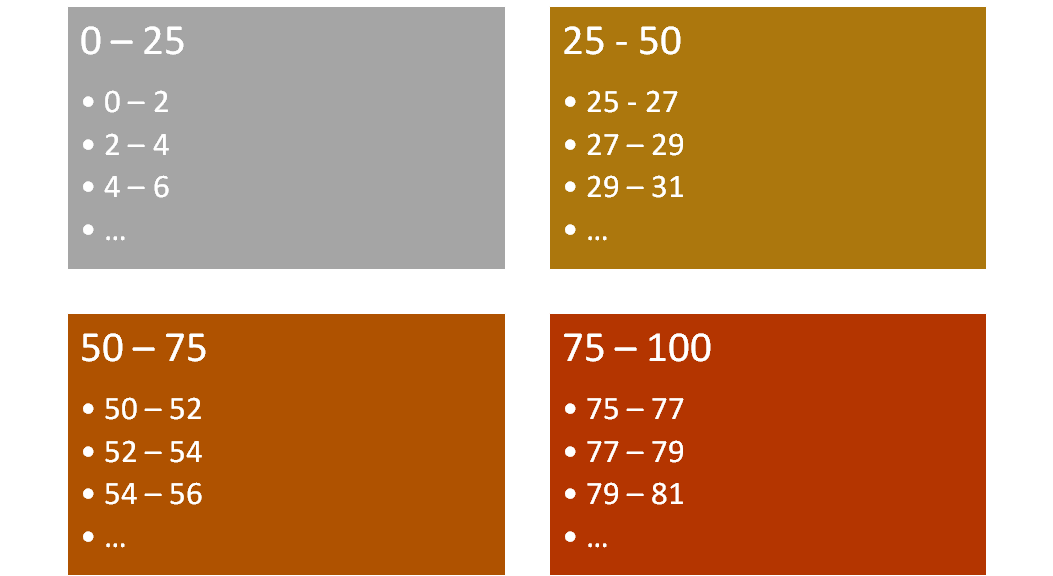
Instead, we can do something like this, let us imagine that you have a machine with 4 cores on it, and the previous mention setup. And then you start 4 threads (each marked with a different color on the image, and start processing nodes.

However, there is a trick here, each thread has a queue, and only ids that fall without the area of responsibility of the thread will arrive there. But we aren’t done, inside a thread we define additional regions, and route requests to process each region into each own queue.

Finally, within each thread, we process one region at a time. So the idea is that while we are running over a region, we may produce work that will need to run on other regions (or even other threads), but we don’t care, we queue that work and continue emptying the work that exists on our own region. Only once once we have completed all work in a particular region will we move to the next one. The whole task complete when, in all threads, there are no more regions with work to be done.

Note that the idea here is that each thread is working on one region at a time, and that region maps to a section of the database file that was memory mapped. So we keep that are of the page cache alive and well.

When we move between regions, we can hint to the memory manager that we are going to need the next region, etc. We can’t escape the need to process the same region multiple times, because processing in one region may lead us to processing in another, and then back, but assuming we run the regions using least recently accessed, we can take advantage on the stuff remaining in the page cache (hopefully) from the previous run and using that.

Which is why the physical location on disk is important.

Note that the actual query that we run is less important. Typical graph queries are fall into one of two categories:

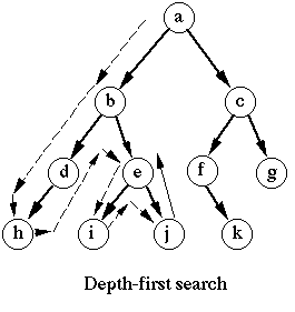
• Some sort of Breadth First Search or Depth First Search and walking through the graph. 
• Finding a sub-graph in the larger graph that matches this criteria.

In both cases, we can process such queries using the aforementioned process, and the reduction in random work that the database has to do is big.

A few posts ago, I talked about the problem of having unstable ids, in particular, ids that can be reused. That leads to quite a lot of complexity, as anyone who ever had to deal with Lucene documents ids knows.

So we are willing to pay something toward stable ids, the questions is what?

One way of doing that is to just store the physical id (unstable) and a virtual id (stable) in a B+Tree (actually, a pair of them, since you’ll need to refer to them back and forth). That means that for the most part, internally to the engine, we’ll use the physical id (with its nice property of having O(1) access time), but externally we’ll expose the stable virtual id (probably sequential numbering, since that is easiest).

Note that I still want to use the physical ids, I’ll discuss exactly why that is important in my next post, for now, let us just say that it is an important component of ensuring high performance for large datasets.

The problem with using B+Tree is that the cost of finding the virtual <—> physical id mapping is O(logN), which for 10 million nodes and 100 million edges is 23 & 24 respectively. Except that this isn’t the real cost function for B+Tree.

Assuming that we have 255 items per page, we actually would need to do 4 page lookups, and a total of 54 comparisons to find the right value. For the edges, we would need 5 page look ups and over 60 comparisons.  Note that this isn’t an issue on its own, but it is an issue when we are talking about having this kind of cost in the hot path of the application. And this is very likely going to be in the hot path.

Oh, there are ways around it, we can only translate back and forth at the edges of the database, so internally we’ll always use the physical address, and only translate it out when we are done. But that is hard to actually do properly, since you need the virtual address for a whole lot of stuff all over the place.

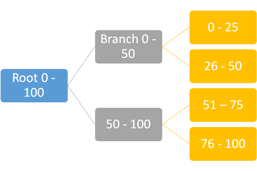
We can steal the idea of page translation tables from the processor. Something like this:

Effectively, we’ll lazy allocate segments of pages and pull them together into a hierarchy. So finding out the physical address of id 84 would involve looking at the root, finding the next page down with mod operation, and so forth until we find the right value and check there. This has the advantage of being simple, O(1) and obvious. It is also pretty good in terms of space saving, since the virtual id can be “stored” without taking any space (it is the position of the physical id in the “array” we created.

This has one drawback, there is no way to recover space. Because the indexer into this data structure is meaningful, we can’t just compact things. Once space is allocated, that is it.  Now, to be fair, the cost in size here for all 100 million edges is about 0.75 GB, so not meaningful in the long run, but if we have a busy database that always write and delete, we have no way to recover the space.

The “proper” answer, by the way, is to implement an external hash table. That has the property of O(1), can grow and shrink as the amount of data changes. I’m not presenting it here mostly because it is something that we haven’t yet had the need to implement in Voron, so it isn’t something that I can just show and move on. Beside, it is fun to explore all the wrong ways of doing something.

I talked about high level and low level data operations. So far, all we have seen are very low level operations (get node, get edges for, etc).

Let us see how we’ll deal with a bigger challenge. In this case, we want to implement a classic graph operation, doing a depth first search, filtering by both nodes and edges.

Here is how we can implement this:

In the real world, we’ll need quite a bit more. On each node (and edge) we’ll need to decide if to return it from the query, or just traverse through it, etc. And that is just to start with.

But I think this demonstrate the point of how to layer behavior on top of the lower level database operations.

There is one thing that we need to talk about still, this code will actually use a lot of individual transactions, one for each independent operation. That is quite expensive, we can open a single transaction and pass it to the functions we call, so there is just a single cost for the entire duration of the operation.

Other things we can do is to explicitly designate specific scenarios as important and change the design so we can answer them very quickly (as in the O(1) cost for accessing nodes/edge data).

I  keep calling this a toy database, and it is true for more reasons than the code existing mostly as unconnected snippets. When defining the storage layer, I breezed through quite a lot of stuff because they didn’t really matter for the point I was trying to make.

We’ll start with talking about node IDs. When we save a node to the database, we get an int64 ID back. What is that? We know that it gives us an O(1) access time to the node (or the edge data), but that’s about it. Typically, we don’t expose the internal table ID in this manner. Because the ID we get back from the Insert corresponds to the location on the disk where that data exists. So the node ID is something that is arbitrary and doesn’t correlate to anything. It isn’t a sequential number, or something that the user defines, or anything like that.

That can lead to issues. In particular, if you want to look up a node by some property, you need to have a way to do so that will retrieve its ID, and only then you can do graph operations from there. The common solution is to use a Lucene index for searching by the properties and finding the root node(s) and proceed from there.

But what about deletes? Deleting a node is possible, and when you do that, the space that was reserved for that node will be freed, and can be reused, so you’ll have a different node with the same ID. This leads to some awkwardness (you can see that with the Lucene document IDs, which have the same problem, although for very different reasons).

Updates also pose a problem, because if you need to extend the size of the node, it might be relocated, which changes the ID. Deleting is a challenge, because you need to remove the deleted node ID from all the edges that reference it, instead of cleaning it up on the fly.

This leads us to either abstract the physical ID with a virtual one (and pay the O(logN) cost for resolving it) or find a way to deal with the above inside your API.

So now that we know how to store the data, in a way that allows efficient graph traversal, let’s compute some back of the envelope computations for storage costs.

Like any storage system, Voron needs to store some metadata about our data, and sometimes this can be very surprising to people.

Let’s look at each of the items that we store in turn.

• Node data is stored in a table.
• Edge data is stored in a table.
• The edge itself is stored in a B+Tree containing fixed size trees.

A table does a bunch of stuff, including reserving some space on the disk, but we don’t have dynamic tables here, so those costs are relatively fixed.

The cost per item, however, depends on the size of the data. If the data size is less than 2036 bytes, then the cost of storing the data is a 4 bytes overhead. If, however, the size of the data item is higher than 2036, we round it up to 4KB section.

In other words, storing ten million nodes, which measure 1KB in size, will cost us about 40 MB  of overhead (compared to roughly 10 GB of data). However, if the size of the data is 2KB, we need to store them in a full page. The reason for this, by the way, is that we need to balance the cost of insert and the cost of update. So we only modify things on page boundary (in this case, 4KB). If the value is small, we pack multiples of them in a single page, but beyond a certain size, we just allocate dedicated pages for them, and live with a bit of free space in the end.

More interesting is the storage of the edge data, actually. A B+Tree costs a minimum of 4KB, and we have one of these per each of the edge types that we have. In practice, we don’t expect there to be a high number of edge types, and we can readily ignore this as fixed size costs. In most cases, I would be stunned to hear that there is more than a single 4KB page for all your edges types (should be enough for a hundred or so).

What isn’t fixed size is the number of fixed size tree (one per source node) and the number of entries in the fixed size trees (one per connection). The whole reason we have fixed size trees is that they allow us to make efficient use of storage by making assumptions. You can see this in their usage. A fixed size tree has an int64 as the key, and you need to specify upfront how much space you need for the values. That makes it very simple to write.

Fixed size trees actually have two forms, they can be embedded or they can be free floating. That mostly depends on their size. If they are embedded, they are stored inside the parent tree, but if they are too large, we store them in their own page. Embedded usage takes 6 bytes per fixed size tree, we have 8 bytes for the key, and the entry size itself (which in our case is also 8 bytes). So a total of 16 bytes per entry inside the fixed size tree.

What this means, in practice, is that up until the moment a node has more than 254 connections, it can be stored as embedded value. When it goes beyond that, we’ll spill over to a full page and start taking space at 4KB increments.

One thing that I didn’t mention is that we store the fixed size trees (keyed by their source node ID), inside a parent B+Tree. Here we need to track a lot more information (keys and values have different sizes, etc). The overhead cost per entry in a B+Tree is 14 bytes. Add to that the 8 bytes for the source node id, and it comes to 22 bytes per source node.

Given all of those numbers, if we had a graph with 10 million nodes and each node was connected to a 10 other nodes in average, and each node/edge was 0.5KB in size, we would have:

• 5 GB – Nodes data – 10,000,000
• 50 GB – Edges data – 100,000,000
• 80 MB – overhead data for nodes & edges.
• 1.75 GB – edges information about all nodes.

Note that in such a graph, we have 10 million nodes, but a hundred million edges. All of which can fit comfortably into RAM on a good server, and give you blazing good performance.

So far we looked into how we can store the nodes and the edges, and we explored some interesting data structures inside Voron. Now, let’s see how we can traverse the graph.

So getting the node is pretty easy, and remember that to access the table by ID gives us an O(1) cost.

Now, what about finding all the edges from a node?

This is a lot heftier, but let’s try to break it into individual pieces. First, we find the tree holding all the edges of that particular type, then we access (by the ID of the source node) the fixed size tree that holds all the connected nodes and the edge data ID.

Finally, we access the edges data (if it exists) to get the data about the edge itself, after which, we return it all to the caller.

Unlike the previous method, here we can’t claim to have O(1) costs. Instead, our costs are composed of:

1. O(logN) – where N is the number of edges types (typically, very few), to search for the right edges tree.
2. O(logN) – where N is the number of source nodes (typically, very large, but the fixed size trees are very good at being fast, and they don’t have to do much).
3. O(N) – where N is the number of connection between the source node and the destination node.

I’m excluding the cost of loading the edge data, since this is an O(1) operation and is directly relevant to the iteration over all nodes connected to the source node.

Ideally, we can find a way to turn the 2nd operation into an O(1) cost, but that should be more than good enough for the moment.

Now, this just gives us traversal of the nodes, but going from here to Breadth First Search / Depth First Search and doing them well is fairly trivial, although there are a few things that we'll need to talk about, but that would serve as a separate post.

We are going to be using Voron to actually handle the storage of the data. Voron is a low level storage engine, which provide, among other things, fully ACID, MVCC and high performance.

For today, what'll look at are the following operations:

• Add a node.
• Add an edge between two nodes.
• Traverse from a node to all its edges (cheaply)
• Traverse from an edge to the other node (cheaply).

Here is the interface code that we will need to build:

I tried to make it as simple as it possible could be. I’m using NameValueCollection because it is a trivial property bag to serialize / deserialize without bringing any additional dependencies.

Let us focus on the initialization of this class. We need to create a StorageEnvironment in Voron, and setup some structures.

Voron has several different storage options for data, and in this case, we are using a table. A table (which is very much unlike a RDMBS table) it a way to store records that has some indexes, but in this case, we are doing something strange. We are defining a table that has no indexes (this is so strange that we need to explicitly allow it). This is useful because tables manages indexes for us automatically, but in this case we will use them strictly for storage. We’ll see why in just a bit.

The code here is a bit strange. Tables are actually meant to hold multiple values, and define indexes on this. So using them to store a single value is something that you wouldn’t normally do. Except that the id that we get back from the table has a very interesting property. It has O(1) cost of access. So given a node id, I can access it directly, regardless of how big my database is. That is a property that I want, because effectively random access of nodes is something that happens quite a lot and is highly desirable.

Now, let us see how we can connect two edges, shall we. This code ignores all error handling, missing nodes, etc. It is meant to explain the core stuff, this is a toy database, after all.

Here we continue doing strange stuff. We already know that we use the empty schema table to have an O(1) access to data. And we store the edge’s data there. But then we run into some new stuff. We create a B+Tree called “Edges_”+type, which hold all of the edges of a particular type. But the content of this B+Tree is not simple. Instead, it is using fixed size trees. Those are also B+Trees, but they have well known size both for keys (which must be long) and the value (which must be small < 256 bytes). Because they are very compact, we can pack quite a lot of data into them, and work with them efficiently.

The end result is that we are now storing the node data and access it at O(1) cost. We also store a B+Tree full of fixed size tree (whose name is the source node id) and whose keys are the destination nodes, and the values are the edge data.

Confusing yet? Not much different than Dictionary<SourceNodeId, Dictionary<DestinationNodeId, EdgeDataId>>. That is quite enough for today, tomorrow I’ll show how we can traverse the data, and what kind of costs are associated with it.

In the Guts n’ Glory of Database Internals posts series (which I’ll probably continue if people suggest new topics), I talked about the very low level things that are involved in actually building a database. From how to ensure consistency to the network protocols. But those are very low level concerns. Important ones, but very low level. In this series, I want to start going up a bit in the stack and actually implement a toy database on top of real production system, to show you what the database engine actually does.

In practice, we divide the layers of a database engine this way:

1. Low level storage (how we save the bits to disk), journaling, ACID.
2. High level storage (what kind of storage options do we have, B+Tree, nested trees, etc).
3. Low level data operations (working on a single item at time).
4. High level data operations (large scale operations, typically).
5. Additional features (subscribing to changes, for example).

In order to do something interesting, we are going to be writing a toy graph database. I’m going to focus on levels 3 & 4 here, the kind of data operations that we need to provide the database we want, and we are going to build over pre-existing storage solution that handles 1 & 2.

Selecting the storage engine – sometimes it make sense to go elsewhere for the storage engine. Typical examples includes using LMDB or LevelDB as embedded databases that handles the storage, and you build the data operations on top of that. This works, but it is limiting. You can’t do certain things, and sometimes you really want to. For example, LMDB supports the notion of multiple trees (and even recursive trees), while LevelDB has a flat key space. That has a big impact on how you design and build the database engine.

At any rate, I don’t think it will surprise anyone that I’m using Voron as the storage engine. It was developed to be a very flexible storage engine, and it works very well for the purpose.

We’ll get to the actual code in tomorrow’s post, but let’s lay out what we want to end up with.

• The ability to store nodes (for simplicity, a node is just an arbitrary property bag).
• The ability to connect nodes using edges.
  • Edges belong to types, so KNOWS and WORKED_AT are two different connection types.
  • An edge can be bare (no properties) or have data (again, for simplicity, just arbitrary property bag)

The purpose of the toy database we build is to allow the following low level operations:

• Add a node.
• Add an edge between two nodes.
• Traverse from a node to all its edges (cheaply)
• Traverse from an edge to the other node (cheaply).

That is it, should be simple enough, right?