This post asked an interesting question, why are hash table so prevalent for in memory usage and (relatively) rare in the case of databases. There is some good points in the post, as well as in the Hacker News thread.

Given that I just did a spike of persistent hash table and have been working on database engines for the past decade, I thought that I might throw my own two cents into the ring.

B+Tree is a profoundly simple concept. You can explain it in 30 minutes, and it make sense. There are some tricky bits to a proper implementation, for sure, but they are more related to performance than correctness.

Hash tables sounds simple, but the moment you have to handle collisions gracefully, you are going to run into real challenges. It is easy to get into nasty bugs with hash tables, the kind that silently corrupt your state without you realizing it.

For example, consider the following code:

This is a hash table using linear addressing. Collisions are handled by adding them to the next available node. And in this case, we have a problem. We want to put “ghi” in position zero, but we can’t, because it is already full. We move it to the first available location. That is well understood and easy. But when we delete “def”, we remove the entry from the array, but we forgot to do fixups for the relocated “ghi”, that value is now gone from the table, effectively. This is the kind of bug you need the moon to be in a certain position while a cat sneeze to figure out.

A B+Tree also maps very nicely to persistent model, but it is entirely non obvious how you can go from the notion of a hash table in memory to one on disk. Extendible hashing exists, and has for a very long time. Literally for more time than I’m alive, but it is not very well known / generically used. It is a beautiful algorithm, mind you. But just mapping the concept to a persistence model isn’t enough, typically, you also had a bunch of additional requirements from disk data structure. In particular, concurrency in database systems is frequently tied closely to the structure of the tree (page level locks).

There is also the cost issue. When talking about disk based data access, we are rarely interested in the actual O(N) complexity, we are far more interested in the number of disk seeks that are involved. Using extendible hashing, you’ll typically get 1 – 2 disk seeks. If the directory is in memory, you have only one, which is great. But with a B+Tree, you can easily make sure that the top levels of the tree will also be memory resident (similar to the extendible hash directory), that leads to typical 1 disk access to read the data, so in many cases, they are roughly the same performance for either option.

Related to the cost issue, you have to also consider security risks. There have been a number of attacks against hash tables that relied on generating hash collisions. The typical in memory fix is to randomize the hash to avoid this, but if you are persistent, you have to use the same hash function forever. That means that an attacker can very easily kill your database server, by generating bad keys.

But these are all relatively minor concerns. The key issue is that B+Tree is just so much more useful. A B+Tree can allow me to:

• Store / retrieve my data by key
• Perform range queries
• Index using a single column
• Index using multiple columns (and then search based on full / partial key)
• Iterate over the data in specified order

Hashes allow me to:

• Store / retrieve my data by key

And that is pretty much it. So B+Tree can do everything that Hashes can, but also so much more. They are typically as fast where it matters (disk reads) and more than sufficiently fast regardless.

Hashes are only good for that one particular scenario of doing lookup by exact key. That is actually a lot more limited than what you’ll consider.

Finally, and quite important, you have to consider the fact that B+Tree has certain access patterns that they excel at. For example, inserting sorted data into a B+Tree is going to be a joy. Scanning the B+Tree in order is also trivial and highly performant.

With hashes? There isn’t an optimal access pattern for inserting data into a hash. And while you can scan a hash at roughly the same cost as you would a B+Tree, you are going to get the data out of order. That means that it is a lot less useful than it would appear to upfront.

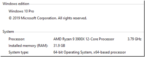
All of that said, hashes are still widely used in databases. But they tend to be used as specialty tools. Deployed carefully and for very specific tasks. This isn’t the first thing that you’ll reach to, you need to justify its use.

One of our developers recently got a new machine, and we were excited to see what kind of performance we can get out of it. It is an AMD Ryzen 9, 12 cores @ 3.79 Ghz with 32 GB of RAM. The disk used was Samsung SSD 970 EVO Plus 500 GB.

This isn’t an official benchmark, to be fair. This is us testing on how fast the machine is. As such, this is a plain vanilla Windows 10 machine, with no effort to perform any optimizations. Our typical benchmark involves loading all of stack overflow into RavenDB, so we’ll have enough data to work with. Here is what things looked like midway through:

As you can see, the write speed we are able to get is impressive.

We were able to insert all of stack overflow, a bit over 52GB in 3 and a half minutes, at a rate of about 300 MB / sec sustained.

Then we tested indexing.

• Map/Reduce on users by registration month (source ~6 million users) – under a minute.
• Full text search on users – two and a half minutes.
• Simple index on questions by tag (over 18 million questions & answers) – 11.5 minutes.
• Full text search on all questions and answers – 33 minutes.

Remember, these numbers are for indexing everything for the first time. It is worth noting that RavenDB dedicates a single thread per index, to avoid hammering the system with too much work. That means that this indexes were building concurrently with one another.

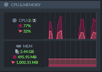
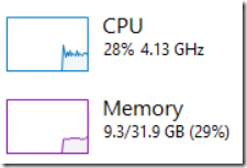
Here is the system utilization while this was going on:

Finally, we tested some other key scenarios (caching disabled in all of them):

• Reading documents (small working set, representing recent questions)  - 243,371 req / ses at 512 MB / sec.
• Full random reads (data size exceed memory, so disk hits) – 15,393.66 res / sec at 13.4 MB / sec.

These two are really interesting numbers. The first one, we generate queries to specific documents over an over (with no caching). That means that RavenDB is able to answer them from memory directly. The idea is to simulate a common scenario of a working set that can fit entirely in memory.

The second one is different. The data size on disk is 52 GB and we have 32 GB available for us. We generate random queries here, for different documents each time. We ensure that the queries cannot be served directly from memory and that RavenDB will have to hit the disk. As you can see, even under this scenario, we are doing fairly well. As an aside, it helps that the disk is good. We tried running this on HDD once. The results were… not nice.

The final test we did was for writes, writing a small document to RavenDB. We got 118,000 writes/sec on a sustained basis, with about 32MB / sec in data throughput. Note that we can do more, but playing with the system configuration, but we are already at high enough rate that it probably wouldn’t matter.

All in all, that is a pretty nice machine.

A map/reduce index in RavenDB can be configured to output its value to a collection. This seems like a strange thing to want to do at first. We already got the results of the index, in the index. Why do we want to duplicate that by writing them to collections?

As it turns out, this is a pretty cool feature, because it enable us to do quite a lot. It means that we can apply anything that work on documents on the results of a map/reduce index. This list include:

• Map/Reduce – so you can create recursive / chained map/reduce operations.
• ETL – so you can push aggregated data to another location, allowing distributed aggregation at scale easily.
• Subscription / Changes – so you can get notified when an aggregated value has been changed.

The key about the list above is that all of them don’t require you to know upfront the id of the generated documents. Indeed, RavenDB uses documents ids like the following for such documents:

Technically speaking, you can compute the id. RavenDB uses a predictable algorithm to generate such an id, but practically speaking, it can be hard to figure out exactly what the inputs are for the id generation. That means that certain document related features are not available. In particular, you can’t easily:

• Include such a document
• Load it directly (you have to query)

So we need a better option to deal with it. The way RavenDB solves this issue is by allowing you to specify a pattern for the output collection, like so:

As you can see, we have a map/reduce index that group by the company and year (marked in blue). We output the collection to YearlySummary, as shown in the previous image.

The pattern (marked in red) specify how we should name the output documents. Here is the result of this index:

And here is what this document looks like:

Huh?

This is strange, you probably think. This is the document we need to show the summary for companies/9-A in 1998, but there is no such data here. Instead, you’ll notice that the document collection is references (marked in red) and that it points to (marked in blue) the actual document with the data. Why do we do things this way?

A map/reduce document is free to output multiple results for the same reduce key, so we need to handle multiple documents here. We also have to deal with multiple reduce outputs that end up with the same pattern. For example, if we use map/reduce by day, but our pattern only specify the month, we’ll have multiple reduce keys that end up with the same pattern.

In practice, because RavenDB has great support for following documents by id, it doesn’t matter. Here is how I can use this index in a query:

This single query allow us to ask a question about companies (those that reside in London, in this case), as well as sales total data for a particular year. Note that this doesn’t do any joins or anything expensive. We have the information at hand, and can just use it.

You’ll notice that the pattern we specified is using both items that we reduce by. But that isn’t mandatory. We can also use this:

Here we only specify the company in the pattern. What would be the result?

Now we get the sales total for the company, on a per year basis.

We can now run the following query:

And this will give us the following output:

As you can imagine, this opens up quite a few possibilities for advanced features. In particular, it means that you can make it even easier for you to show and process aggregate information and work through complex object models.

Exactly 9 years ago, Hibernating Rhinos had a major breakthrough. We moved to our own offices for the first time. Before that, I was mostly working from a home office of clients’ locations.  Well, I say we, but I mean I. At the time, the change mostly involved me having to put on some shoes and going out of the house to work alone in a big empty office. The rest of the team at the time was completely remote.

I got the office because I needed to. Some people can manage a proper life / work balance while working from home. I find it very hard. I’m the kind of person that would get up at 2 AM to get something to drink, see a new mail notification on the monitor, and start working until 8 AM. Having a separate office was hugely beneficial for me.  The other reason was that it allowed me to hire more people locally. The first real employee I had was hired within three months of moving to the new office.

That first office was great, but small. Just 5 rooms about about 120 m² (1300 ft²). We stayed in the office until we got to about 12 people. At this point, we really didn’t have enough room to swing a cat (to be fair, we didn’t have an office cat, nor a real good reason to want to swing one). We moved offices in 2015, from the center of the industrial zone of the city to the periphery of the business zone). The new offices were 250 m² (2700 ft²) and gave us a lot of room to expand, it also had two major advantages. It was nice to be able to walk downstairs and be able to walk to pretty much anywhere we needed to and we no longer had to deal with having a garage next door.

When we moved to the 2nd office, it felt like we had a huge amount of room, but it filled up quite quickly. It was certain that we would outgrow the new place in a short order, so we started looking for a permeant home that would suffice for the next 10 years or so. We got one, smack down in the center of the business zone of the city. Next door to city hall, actually. Well, I say “got one”. What we actually got was a piece of paper and a hole in the ground. Before we could move into the new offices, they had to be built first.

We stayed in the second office space for 3 years, but we run out of room before the new offices were ready. So we moved for the third time. Because our new offices weren’t ready, we moved to a shared working space (like WeWork). We planned on being there for a short while, but it ended up for over a year. The plus side, we were able to expand much more easily. We hired quite a few people this year and was able to simple add more offices as we grew. The down side was that this is very much not our office, so we really want to move.

This week, however, we are going to finally move. The new offices have more than enough space  415 m² (4500 ft²) for the new five to ten years of growth, it covers two floors in a brand new location, centrally located and beautifully done. I’m not posting any pictures because the vast majority of our own team haven’t seen it yet (we have a unveiling party tomorrow), but I’m super happy that we got to this point and just had to share in the blog.

We have just rolled out GCP support for RavenDB Cloud. The support is still in the beta stage, because we like to be conservative, but you now have the ability to deploy RavenDB clusters on GCP at the click of a button.

All the usual features are supported. You can provision a new cluster, RavenDB Cloud will monitor and manage it for you, and you can focus on deliver actual value, instead of deployment concerns. As usual with RavenDB Cloud, we are deployed to all public regions in GCP.

For the beta period, we only support production clusters (no single development instances) on GCP.

As usual, we would love to have your feedback.

We got an interesting question in the mailing list. Given the following documents structures:

We want to be able to merge these into the following output:

If we had just a single skill in the professions document, that would have been easy. It would also be easy if we had the professions recorded in the skills document. But we have to merge multiple separate skills, without knowing what professions they belong to. RavenDB doesn’t support doing this directly, so we have to do a bit of work to do so.

We can easily merge documents in RavenDB if we have the document id of the relevant document. But in this case, the external id of the skill isn’t part of the document id, so that complicate things.

The very first thing we need to do is to allow ourselves to reference a skill by its external id. This is done by creating a map/reduce index that project the value out, like so:

Note that we specify a pattern for the collection references, based on the actual data from the document. The index itself doesn’t really do much, to be fair, just gives me the document id we wanted to. I’ll post about this feature more in the next post, for now, I’m just using this to generate the results I want. Here is the generated document:

Because there may be multiple documents with the same value, we don’t end up with the actual document, but with a middle man that point to all the matches.

And here we have the reference to the original document, so we can now start working. We need another index, to bring it all together:

There is a lot going on here, it seems. But we are simply walking the line of documents, to find all the documents that we need. And here is the final result:

The nice thing about all this work is that this happens at indexing time. Meaning that queries on this data is really fast.

My webinar about From Monolith to Microservices: Scaling out Your Architecture is now up

As usual, I would love your feedback

An old adage about project managers is that they are people who believe that you can get 9 women together and get a baby in a single month. I told that to my father once and he laughed so much we almost had to call paramedics. The other side of this saying is that you can get nine women and get nine babies in nine months. This is usually told in terms of latency vs. capacity. In other words, you have to wait for 9 months to get a baby, but you can get any number of babies you want in 9 months. Baby generation is an embarrassingly parallel problem (I would argue that the key here is embarrassingly). Given a sufficient supply of pregnant women (a problem I’ll leave to the reader), you can get any number of babies you want.

We are in the realm of project management here, mind, so this looks like a great idea. We can set things up so we’ll have parallel work and get to the end with everything we wanted. Now, there is a term for nine babies, is seems: nonuplets.

I believe it is pronounced: No, NO, @!#($!@#.

A single baby is a lot of work, a couple of them is a LOT of work, three together is LOT^2. And I don’t believe that we made sufficient advances in math to compute the amount of work and stress involved in having nine babies at the same time. It would take a village, or nine.

This is a mostly technical blog, so why am I talking about babies? Let’s go back to the project manager for a bit? We can’t throw resources at the problem to shorten the time to completion (9 women, 1 month, baby). We can parallelize the work (9 women, 9 months, 9 babies), though. The key observation here, however, is that you probably don’t want to get nine babies all at once. That is a LOT of work. Let’s consider the point of view of the project manager. In this case, we have sufficient supply of people to do the work, and we have 9 major features that we want done. We can’t throw all the people at one feature and get it down in 1 month. See, Mythical Man Month for details, as well as pretty much any other research on the topic.

We can create teams for each feature, and given that we have no limit to the number of people working on this, we can deliver (pun intended) all the major features at the right time frame. So in nine months, we are able to deliver nine major features. At least, that is the theory.

In practice, in nine months, the situation for the project is going to look like this:

In other words, you are going to spend as much time trying to integrate nine major features as you’ll be changing diapers for nine newborn babies. I assume that you don’t have experience with that (unless you are working in day care), but that is a lot.

Leaving aside the integration headache, there are also other considerations that the project manager needs to deal with. For example, documentation for all the new features (and their intersections).

Finally, there is the issue of marketing, release cadence and confusion. If you go with the nine babies / nine months options, you’ll have slower and bigger releases. That means that your customers will get bigger packages with more changes, making them more hesitant to upgrade. In terms of marketing, it also means that you have to try to push many new changes all at once, leading to major features just not getting enough time in the daylight.

Let’s talk about RavenDB itself. I’m going to ignore RavenDB 4.0 release, because that was a major exception. We had to rebuild the project to match a new architecture and set of demands. Let’s look at RavenDB 4.1, the major features there were:

1. JavaScript indexes
2. Cluster wide transactions
3. Migration from SQL, MongoDB and CosmosDB
4. RavenDB Embedded
5. Distributed Counters

For RavenDB 4.2, the major features were:

1. Revisions Revert
2. Pull Replication
3. Graph queries
4. Encrypted backups
5. Stack trace capture on production

With five major features in each release (and dozens of smaller features), it is really hard to give a consistent message on a release.

In software, you don’t generally have the concept of inventory: Stuff that you already paid for but haven’t yet been sold to customers. Unreleased features, on the other hand, are exactly that. Development has been paid for, but until the software has been released, you are not going to be able to see any benefits of it.

With future releases of RavenDB, we are going to reduce the number of major features that we are going to be working on per release. Instead of spreading ourselves across many such features, we are going to try to focus on one or two only per release. We’re also going to reduce the scope of such releases, so instead of doing a release every 6 – 8 months, we will try to do a release every 3 – 4.

For 5.0, for example, the major feature we are working on is time series. There are other things that are already in 5.0, but there are no additional major features, and as soon as we properly complete the time series work, we’ll consider 5.0 ready to ship.

A common question I field on many customer inquiries is comparing RavenDB to one relational database or another. Recently we got a whole spate of questions on RavenDB vs. PostgreSQL and I though that it might be easier to just post about it here rather than answer the question each time. Some of the differences are general, for all or most relational databases, but I’m also going to touch on specific features of PostgreSQL that matter for this comparison.

The aim of this post is to provide highlights to the differences between RavenDB and PostgreSQL, not to be an in depth comparison of the two.

PostgreSQL is a relational database, storing the data using tables, columns and rows. The tabular model is quite entrenched here, although PostgreSQL has the notion of JSON columns. 

RavenDB is a document database, which store JSON documents natively. These documents are schema-free and allow arbitrarily complex structure.

The first key point that distinguish these databases is with the overall mindset. RavenDB is meant to be a database for OLTP systems (business applications) and has been designed explicitly for this. PostgreSQL is trying to achieve both OLTP and OLAP scenarios and tends to place a lot more emphasis on the role of the administrator and operations teams. For example, PostgreSQL requires VACUUM, statistics refresh, manual index creation, etc. RavenDB, on the other hand, it design to run in a fully automated fashion. There isn’t any action that an administrator needs to take (or schedule) to ensure that RavenDB will run properly.

RavenDB is also capable of configuring itself dynamically, adjusting to the real world load it has based on feedback from the operational environment. For example, the more queries a particular index has, the more resources it will be granted by RavenDB. Another example is how RavenDB processes queries in general. Its query analyzer will run through the incoming queries and figure out what is the best set of indexes that you need to answer them. RavenDB will then go ahead and create these indexes on the fly. Such an action tends to be scary for users coming from relational databases, but RavenDB was designed upfront for specifically these scenarios. It is able to build the new indexes without adding too much load to the server and without taking any locks. Other tasks that are typically handled by the DBA, such as configuring the system, are handled dynamically by RavenDB based on actual operational behavior. RavenDB will also cleanup superfluous indexes and reduce the resources available for indexes that aren’t in common use. All of that without a DBA to perform acts of arcane magic.

Another major difference between the databases is the notion of schema. PostgreSQL requires you to define your schema upfront and adhere to that. The fact that you can use JSON at times to store data provides an important escape hatch, but while PostgreSQL allows most operations on JSON data (including indexing them), it is unable to collect statistics information on such data, leading to slower queries. RavenDB uses a schema-free model, documents are grouped into collections (similar to tables, but without the constraint of having the same schema), but have no fixed schema. Two documents at the same collection can have distinct structure.  Typical projects using JSON columns in PostgreSQL will tend to pull specific columns from the JSON to the table itself, to allow for better integration with the query engine. Nevertheless, PostgreSQL’s ability to handle both relational and document data gives it a lot of brownie points and enable a lot of sophisticated scenarios for users.

RavenDB, on the other hand, is a pure JSON database, which natively understand JSON. It means that the querying language is much nicer for querying that involve JSON and comparable for queries that don’t have a dynamic structure. In addition to being able to query the JSON data, RavenDB also allows you to run aggregation using Map/Reduce indexes. These are similar to materialized views in PostgreSQL, but unlike those, RavenDB is going to update the indexes automatically and incrementally. That means that you can query on large scale aggregation in microseconds, regardless of data sizes.

For complex queries, that touch on relationships between pieces of data, we have very different behaviors. If the relations inside PostgreSQL are stored as columns and using foreign keys, it is going to be efficient to deal with them. However, if the data is dynamic or complex, you’ll want to put it in a JSON column. At this point, the cost of joining relations skyrockets for most data sets. RavenDB, on the other hand, allow you to follow relationships between documents naturally, at indexing or querying time. For more complex relationships work, RavenDB also has graph querying which allow you to run complex queries on the shape of your data.

I mentioned before that RavenDB was designed explicitly for business applications, that means that it has a much better feature set around their use case. Consider the humble Customers page, which needs to show the Customers details, Recent Orders (and their total), Recent Support Calls, etc.

When querying PostgreSQL, you’ll need to make multiple queries to fetch this information. That means that you’ll have to deal with multiple network roundtrips, which in many cases can be the most expensive piece of actually querying the database. RavenDB, on the other hand, has the Lazy feature, which allow you to combine multiple separate queries into a single network roundtrip. This seemingly simple feature can have a massive impact on your overall performance.

A similar feature is related to the includes feature. It is very common when you load one piece of data that you want to get related information. With RavenDB, you can indicate that to the database engine, which will send you all the results in one shot. With a relational database, you can use a join (with the impact on the shape of the results, Cartesian products issue and possible performance impact) or issue multiple queries. Simple change, but significant improvement over the alternative.

RavenDB is a distributed database by default while PostgreSQL is a single node by default. There exists features and options (log shipping, logical replication, etc), which allow PostgreSQL to run as a cluster, but they tend to be non trivial to setup, configure and maintain. With RavenDB, even if you are running a single node, you are actually running a cluster. And when you have multiple nodes, it is trivial to join them into a cluster, from which point on, you can just manage everything as usual. Features such as multi-master, the ability for disconnected work and widely distributed clusters are native parts of RavenDB and integrate seamlessly, while they tend to be of the “some assembly required” in PostgreSQL.

The two databases are very different from one another and tend to be used for separate purposes. RavenDB is meant to be the application database, it excels in being the backend of OTLP systems and focus on that to the exclusion of all else. PostgreSQL tend to be more general, suitable for dynamic queries, reports and exploration as well as OLTP scenarios. It may not be a fair comparison, but I have literally built RavenDB specifically to be better than a relational database for the common needs of business applications, and ten years in, I think it still shows significant advantages in that area.

Finally, let’s talk about performance. RavenDB was designed based on failures in the relational model. I spent years as a database performance consultant, going from customer to customer fixing the same underlying issues. When RavenDB was designed, we took that to account. The paper OLTP – Through the Looking Glass, and What We Found There has some really interesting information. Including the issue of about 30% of a relational database performance is spent on locking.

RavenDB is using MVCC, just like PostgreSQL. Unlike PostgreSQL, RavenDB doesn’t need to deal with transaction id wraparound, VACUUM costs, etc. Instead, we maintain MVCC not on the row level, but on the page level. There is a lot less locks to manage and deal with and far less complexity internally. This means that read transactions are completely lock free and don’t have to do any coordination with write transactions. That has an impact on performance and RavenDB can routinely manage to achieve benchmark numbers on commodity hardware that are usually reserved for expensive benchmark machines.

One of our developers got a new machine recently and did some light benchmarking. Running in WSL (Ubuntu on Windows), RavenDB was able to exceed 115,000 writes / sec and 275,000 reads / sec. Hare the specs:

And let’s be honest, we weren’t really trying hard here, but we still got nice numbers. A lot of that is by designing how we interact internally to have a much simpler architecture and shape, and it shows. And the nice thing is that these advantages are cumulative. RavenDB is fast, but you also gain the benefits of the protocol allowing you to issue multiple queries in a single roundtrip, the ability to include additional results and dynamically adjusting to the operation environment.

It Just Works.

After a long journey, I have an actual data structure implemented. I only lightly tested it, and didn’t really do too much with it. In fact, as it current stands, I didn’t even implement a way to delete the table. I relied on closing the process to release the memory.

It sounds like a silly omission, right? Something that is easily fixed. But I run into a tricky problem with implementing this. Let’s write the simplest free method we can:

Simple enough, no? But let’s look at one setup of the table, shall we?

As you can see, I have a list of buckets, each of them point to a page. However, multiple buckets may point to the same page. The code above is going to double free address 0x00748000!

I need some way to handle this properly, but I can’t actually keep track of whatever I already deleted a bucket. That would require a hash table, and I’m trying to delete one . I also can’t track it in the memory that I’m going to free, because I can’t access it after free() was called. So what to do?

I thought about this for a while, and I came up with the following solution.

What is going on here? Because we may have duplicates, we first sort the buckets. We want to sort them by the value of the pointer. Then we simply scan through the list and ignore the duplicates, freeing each bucket only once.

There is a certain elegance to it, even if the qsort() usage is really bad, in terms of ergonomics (and performance).