Oren Eini

CEO of RavenDB

a NoSQL Open Source Document Database

Get in touch with me:

oren@ravendb.net +972 52-548-6969

Posts: 7,523
|
Comments: 51,145
Privacy Policy · Terms
filter by tags archive
time to read 2 min | 344 words

As the final post in this series, I decided to see how I can create a complex query. Given the NSA’s statement, I decided to see if I can use LemonGraph to find a dog of interest. In particular, given our graph, I wanted to find start with a particular dog and find another dog that likes this dog that also like a dog that dislike the original.

As a reminder, here is the graph:

image

And starting from Arava, I want to find a dog that likes Arava that also likes a dog that isn’t liked by Arava.

The LemonGraph query language isn’t very expressive, or at least I’m not familiar enough with it to make it work properly. I decided on the following query:

n(type="dog", value="arava")->
               @e(type="likes", value="yes")->
n(type="dog")->
               @e(type="likes", value="yes")->
n(type="dog")->
               @e(type="likes", value="no")->
@N(type="dog", value="arava")

This is a bit of a brute force method to do this. It encodes the path directly. There are a few minor things that might not be obvious here. The @ prefix means don’t return this to the user and the N() indicates that we shouldn’t filter already seen values. I can certainly see how this can be useful for certain things Smile. I wonder if LemonGraph has a better way to express such a query.

This is the first time I actually reviewed this kind of codebase, where some things are done in C and some in Python. It was quite interesting to see the interaction between them. The codebase itself is really interesting, but I found it really hard to follow at times. The love affair with tuples and dynamic behavior made the code non trivial and likely is going to cause maintenance issues down the line. It is also quite obvious that this is intended for internal consumption, with very little time or effort spent on “productization”. By that I meant things like better query errors and more obvious thing to do.

It has an interesting approach to solving the problem of graph queries and I’ve learned quite a few things from it.

time to read 7 min | 1300 words

After going over many layers inside LemonGraph, I think we are ready to get to the real deal. We know how LemonGraph starts to execute a query. It find the clause that is likely to have the least number of items and starts from there. These are the seeds of the query, but how is it going to actually process that?

Here is my graph:
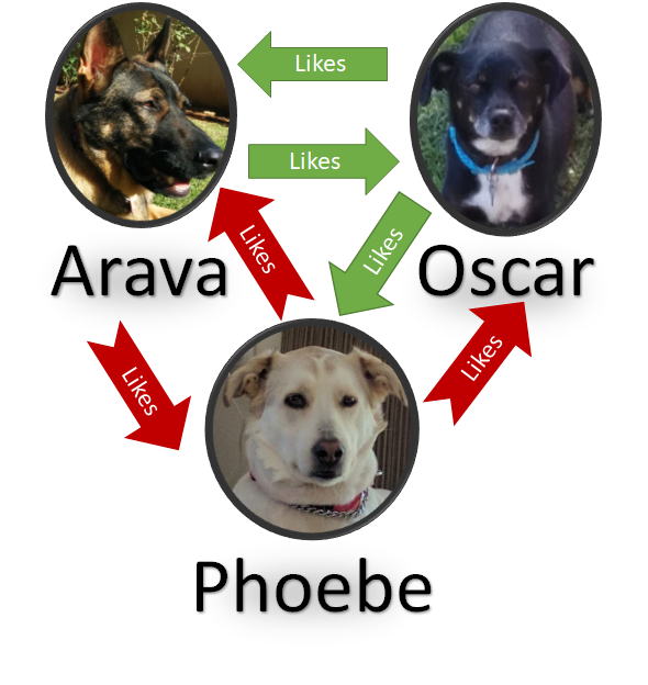
image

And here is the query that I want to run on it: n()->e(type="likes", value="yes")->n()

LemonGraph detects that the cheapest source of seeds for this query is the edge and provides these to the MatchCTX class which does the actual processing. Let’s explore how it is working on a single seed.

The actual behavior starts from the matches() method, which starts here:
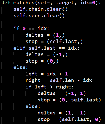
image

As usual for this codebase, the use of tuples for controlling behavior is prevalent and annoying. In this case, the idx argument controls the position of the target in the query, whatever this is the start, end or somewhere in the middle. The deltas define what direction the matches should go and the stops where you must stop searching, I think.

Now that we setup the ground rules, the execution is as follows:

image

In this case, because the seed of our query is the edge (which is in the middle) it determines that deltas are (1, –1) and stops are (2, 0). We’ll also go to the first clause in the if statement. The link variable there controls whatever we should follow links going in or out.

There is a lot of logic actually packed into the link initialization. The self.link is an array that has ‘next’ and ‘prev’ as its values, so the idea is that it find what property to look at, then use the dictionary syntax to get the relevant property and decide what kind of direction it should go.

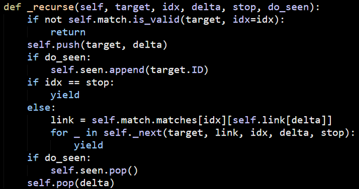
We’ll focus on the _recurse() method for now. In this case, we are being passed:

  • idx = 1
  • delta = 1
  • stop = 2

Here is the actual method:

image

As you can see, we first validate that the match is valid (this is where we mostly check other properties of the value that we are currently checking, filtering them in place). Usually the do_seen will be set to True, which will ensure that we only traverse each node once. The main iteration logic is done in combination with the _next() method, shown below:
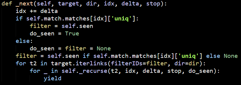
image

The first line there shows usage of delta, which control in what direction to move. I’m not quite sure why the filter is set in the if statements, since it is also being set immediately after. This looks like redundant code that snuck in somehow.

The bulk of the work is shelled out to iterlinks, so let’s check what is going on there… I know that we are running on an edge here, so we need to look at the Edge.iterlinks() method:
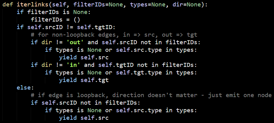
image

There isn’t really much to tell here, it checks the filters and return the incoming or outgoing edges, nothing more. On the other hand, the Node.iterlinks() implementation is a bit simpler:image

We’ll explore exactly how the edges are loaded for a node in a bit, however, I do want to note right now that the _next() method isn’t passing the types of the edge, even though it looks to me that it has this information. In that case, that would give a performance boost because it could filter a lot of edges in busy graphs.

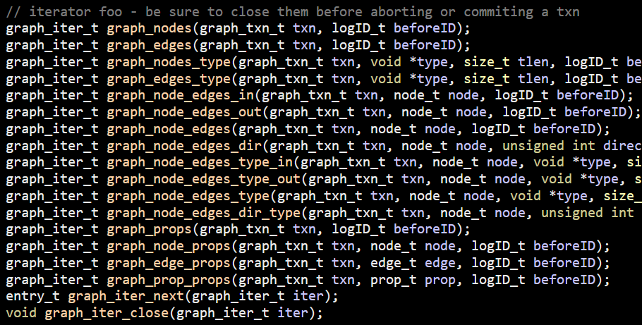
Actually, I already looked at how iterators working in a previous post, so I won’t go over all of that again. This is basically calling this method

image

The graph_node_edges_in() and graph_node_edges_out() methods are pretty simple, basically just scanning the DB_TGTNODE_IDX or DB_SRCNODE_IDX indexes, respectively. The graph_node_edges() however, is really strange.

Here it is:

image

It took me a few reads to figure out that this is probably a case of someone unpacking a statement for debugging but forgetting to remove the packed statement. The second return statement is ignored and likely stripped out as unreachable, but it is pretty confusing to read.

The graph_iter_concat() answers a question I had about how graph_iter_t is used, here is how it looks like:
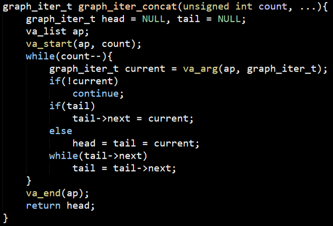
image

This is using C’s support for passing an unknown number of parameters to a method. This basically builds a simple linked list, which also answers the usage of _blarf() function and its behavior a few posts ago.

So we are back were we started, we understand how the data flows into the Python code, now let’s go back and look at _recurse() and _next() calls.

Now I know a lot more about the behavior of the code, so this make sense. The stop argument to the _recurse() control the depth of the number of links that would be traversed in a particular query. Now that I know how this particular clause work, I understand how LemonGraph goes from the edge to the node in e()->n(), but I don’t know how it goes to back to find the full path.

The key for that are the calls to push()  and pop() in the the MatchCtx._recurse() methods. These update the chain, like so:

image

In processing the query, we first append the edge to the chain:

image

The next step goes from the edge to it’s destination, giving us Oscar:

image

Remember that in the matches(), we got into this if clause:

image

This is when we start scanning an edge, which first add things to the right, then it scan things to the left in the _next() method. Look at the push() method there. By the time we get to the result(), we have iterated both sides of the connection, giving us:

image

That is a very clever way of doing things.

Let’s try doing things a little bit differently. I’m going to check a slightly different query: n(type=”dog”, value=”arava”)->e(type="likes", value="yes")->n()

If I understand things correctly, this is going to select the node as the starting point, because that is a lot more efficient. That will allow me to figure out the other side of this operation. I just run this through the debugger, and this is indeed how it actually works.

The usage of yield to pass control midway is not trivial to follow, but it ends up being quite a nice implementation. This is enough for this post. In my next one, I want to explore a few of the possible operations that exposed by LemonGraph.

time to read 6 min | 1089 words

I said before that I don’t want to get into the details of how LemonGraph is dealing with parsing the queries. Unfortunately, I can’t avoid that. There seems to be a lot of logic, magic and mystery in the MatchLGQL() class, which is critical to understanding how queries work.

The problem is that either my Python-fu is lacking or it is just really hard to figure out a non trivial codebase behavior in a dynamic language like python. I find it hard to figure out what data is stored where and how it is manipulated. Therefor, I decided to break with my usual custom and actually run the code in the debugger to try to follow what is going on there. I tried to run this on WSL, but it crashed horribly, so I had to spin up a VM and setup PyCharm on it. First time that I’m actually using that and the experience is pretty nice so far. Being able to inspect things directly means that it is much easier to figure out the behavior of the code.

In order to explore how queries work in LemonGraph, I created the following graph, which represents the relationships between my dogs:

image

Here is how this looks like in code:

This tells us to find all the dogs that like each other. And it finds:

  • Arava –> Oscar
  • Oscar –> Arava
  • Oscar –> Pheobe

Now that we have a query that we can sink our teeth into, let’s figure out how this work, shall we? Inside the dreaded MatchLGQL() class, there are all sorts of regular expressions running on the parse this thing, but eventually we get to the partially processed parsed query:

image

This screen shot might explain why I wasn’t happy with the code structure for figuring out what is going on without debugging. The number of tuples here is quite amazing, and they are used everywhere. This make static analysis (as in, just reading the code) too hard for me. But with the debugger, that is much easier. If you are familiar with ASTs, this should be pretty easy to figure out.

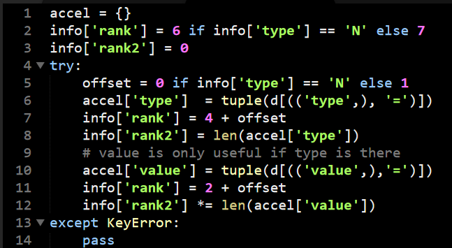
Here is a piece of code that we already looked at (and criticized), this is in munge_obj() method, where it is deciding how to optimize the query:

image

This piece of code is critical for the performance of the system. And it is really hard to understand. Here is what is going on.

The accel array tell a later piece of code how to accelerate the query, using the type or type and value to start from a particular source. The info is used to carry state about particular clause in the query. Before this code run there is some code that builds the dictionary d which is used to figure out the filters on the particular clause. This is fun, because it is using missing a key lookup in the dictionary for control flow.

Let’s follow the logic?

  • Line 2 - If the clause operates on a node, rank it as 6. If it is an edge, rank it as 7.
  • Line 6 – If the clause has a type specified, rank is as 4 if it is a node, 5 if it is an edge. Otherwise, abort the optimization.
    • You might not see the “abort this optimization” in line 6, because it relies on the dictionary to throw if the key isn’t found. This is a common pattern in this code and something that I personally greatly dislike.
  • Line 8 – it uses the length of the type as a metric for secondary ranking. I’m not quite sure why this is the case. I guess the code needed a tie breaker, but I can’t imagine why the length of a type would have any impact on performance.
    • Unless, of course, the code assumes that shorter types are more common, and therefor will prefer to use the rare longer types?
  • Line 10 – If there is a type and a value defined, that is even better. Note that again the is the ranking of node (2) and edge (3) which I find non obvious.

Here are the results of the matches after they have been munged, I marked the ranking:

image

Looking at this, this seems very strange, the rank2 value is 1 in the second element, but I expected it to be the length of the string. As it turns out, this is not working directly on the string, it is working on the tuple of possible values, so the secondary ranking here is not based on the length of the type or the value but on the number of possible types and values that were specified for each clause.

The code judges that the best place to start this query is with the second entry, since it is the most specific option. This in turn takes us the the seeds() method that we previously covered. In this case, the code is going to hit this branch:

image

This means that it is going to be iterating over all the edges of a particular type and filtering them in Python code. This is strange, because the on disk indexes actually support doing a direct query on the (type, value) directly and would probably be much cheaper in the case you have many values for a particular type of an edge.

In fact, just that is implemented for querying nodes by (type, value):

image

I’m guessing that they are either don’t have a lot of queries on (type, value) on edges or not a lot of different values for edge types that they can optimize in this manner.

That is enough for now, I have a pretty good grasp of how queries are parsed and how they fetch data from the underlying storage. The next post will talk about how LemonGraph takes the seeds of the query and execute the actual graph operations on them. The code that does this is tight and will require a full post to explore properly.

time to read 2 min | 244 words

Before going over the actual query implementation, I wanted to talk about something that I just realized. I said previously that I don’t understand why LemonGraph is using its integer encoding method, because it is less efficient than using variant sized integer. What I didn’t take into account is that the method LemonGraph is using gives short, but sortable, integers.

Here is the encoding method:

image

Now, let’s see what kind of binary output this will generate when given a few numbers:

image

The key here is that the number of bytes is stored as the first item. This means that when we compare two numbers using memcmp(), the number with more bytes is considered greater. This is indeed the case, because if you need more bytes to store a number, it is obviously larger.

What about two numbers that have the same number of bytes? This is handled by simple binary comparison of the values. If they are the same size, the fact that the encode() output them in big endian format means that we can compare them using memcmp() and be done with it.

This is a really nice way to both keep the values sorted and to avoid storing the full 8 bytes for numbers that are usually much smaller.

time to read 7 min | 1384 words

After figuring out how LemonGraph is storing data on disk, my next task is to figure out how queries are handled. Here are some queries:

image

A query starts in the Python’s Query class, where it is parsed by the MatchLGQL class. I scanned this code briefly, but this is basically doing query parsing into the in memory representation. This is typically ugly piece of code, and that holds true for this code as well. Python’s dynamic nature also means that there isn’t an easy to follow set of AST classes. I’ll skip the details of query parsing and just see how it is actually handling the queries, then.

I started to look into the query execution and got lost in details that I didn’t understand. In particular, there is a very strong tie between the query parsing and the execution. More so than I expected. What brought this home was this piece of code, which is used to rank the most efficient manner in which you should start executing the query.

image

At this point, I think that the idea here is that when you start running a query, you want to start from the smallest set of seed nodes. the ranking here seems to be a nice way to go about doing just that, but I’m not really sure yet how this is applied.

This is later used to figure out what the best starting location is in the Query.finalize() method.

image

This all come together for me inside the _adhoc() method on Query, where the query is actually being run:

image

The self.compiled is the set of already parsed matches. On each of them, we create a context (which will track already visited nodes / edges) and start by finding the seeds on the query. Seeds are handled using… an interesting approach:

image

It took me a few reads to get what this code is trying to do and I still thing that this is an obnoxious way to write things. This basically does the other side of the ranking. It is using the ranking to decide which method to call. I think that an enum would be about three time more readable. Especially since a bit lower you have:

image

I have to say that the modulus usage is the sign of true genius. Or madness. I’m not sure which, because I can’t figure out what the history of this code is. This was the same way from the initial commit, but I think that this code has history from before the public release. And it might have a reason for this kind of code. But I don’t like it and I think it would have been much easier to read if it wasn’t using magic numbers all over the place.

At any rate, let’s assume that we have the simplest query, for all the nodes. This would send us to txn.nodes() method. This would be rank 6, by the way. Here is how this looks like:

image

As you can see, we have two modes here. If the rank was 6, we aren’t sent a type. But if the rank was 4, we are getting a type. I’m going to start from the search for types, which seems more interesting.

Here is where we end up in the C code:

image

Yes, the graph_nodes_type() method is calling _graph_nodes_edges_type() method. That was confusing as well to me. The key here is the DB_NODE_IDX index there, which tell it to use a different tree for the lookups.

The graph_string_lookup() is something that we already run into, this is the __blob_resolve() method, which is searching for the string id for the given type. The code starts to get interesting when we see the graph_iter_new() call:

image

So we specify an iterator on the given prefix. From the previous post, you might recall that DB_NODE_IDX is specific as (type, val –> id). So this does a search on the first item that matches the prefix.  The _cleanse_beforeID() method will ensure that the beforeID is only valid if it represent a value that is between 1 and the max log id that was generated on the graph.

The iterator we got from the nodes() method just implement’s Python iteration interface, starting from the graph_iter_new() item, then calling graph_iter_next() until the end. This is implemented like so:

image

Here we see for the first time the actual usage of beforeID. I’m not sure what this does yet, so we’ll skip this for now and look at the _iter_idx_nextID() method and come back to it later. This method is quite interesting. We have the head of the iterator, which is set to true in the iterator init. I’m not sure what this means yet. What seems to be interesting is that _blarf() method, which I understand to be a cry of frustration (I had to look it up).

image

I’m not sure what the next pointer is doing there at all. We’ll look at that after I’ll inspect (with some measure of dread) the _blarf() function.

image

To start with, I love the use of goto instead of return statements. I understand that this may be a coding convention here and this is used to clearly mark when resources are supposed to be disposed, but still…

The iter_next_key() ends up moving the cursor (and validating that the prefix is still valid). The _parse_idx_logID() call is here:

image

And this is just a fancy way of saying, gimme the last value in this buffer.

To understand what is going on, let’s go back a bit and understand what is going on here. We are actually scanning the index DB_NODE_IDX. And that index has the value of (type, val, id). Since the iteration is done in sorted order, this means that you can iterate over all the matches that match the type you want. The use of beforeID for filtering here, however, is interesting. I wonder how common is the use of historical queries like this are. Because if you need to skip over a lot of items, this will result in an O(N) operation while you are scanning and discarding a lot of data.

Anyway, there doesn’t seem to be any use of the graph_iter_t.next in this code path, so I’ll leave it for now. The iteration over all the nodes is done with the exact same method, but without specifying any prefix, which means that it matches everything.

I have to admit that at this point, I don’t really get how it process the more complex queries. I had to give up the “let’s not run the code” and try a few things out. Surprisingly, on WSL, the code just cause segmentation fault. I tracked it down to something in cffi, but I didn’t care that much. I created a simple ubuntu machine and played with it for a bit. So far, we just looked at how we get the first seeds of the query. A lot of the smarts seems to be hidden in the MatchCTX class.  In particular, the matches() method seems to be doing a lot of magic.

I’m going to concentrate on that in my next post.

time to read 3 min | 546 words

The last post left us figuring out how LemonGraph is storing nodes and edges. There are the special properties type and val that are used for this kind of lookup. I find it interesting that these two properties are treated in a special manner. It seems like it would be more useful to have such distinction completely arbitrary or use a single property. A more common approach would be to just have a unique key for each node / edge and be done with it. I’m guessing that this is needed because you might want to do partial searches. So give me all the nodes whose type is X without caring what the value is.

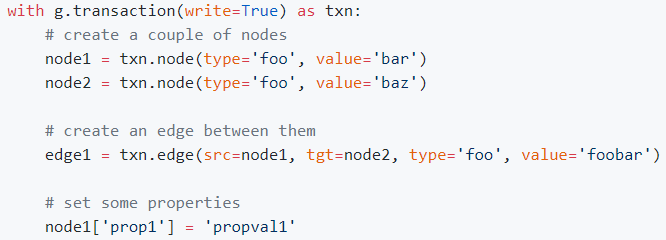
Here is the sample code from the project’s page:

image

In the last post, I was able to follow up on the first two lines. Now, let’s see how the edge is actually used and how properties are stored. The edge() method call ends up calling the __edge_resolve() method:

image

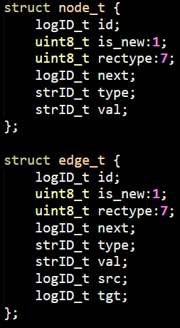
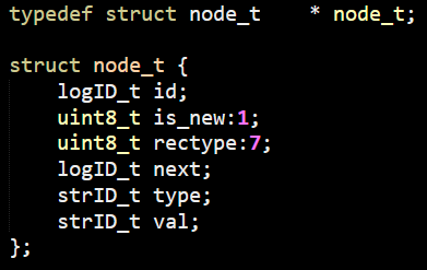
This is very similar to what we saw with __node_resolve() method. This might be a good time to stop and consider the edge_t and node_t structures:

image

They seems pretty simple. The is_new:1 syntax is used by C for bitfields. In other words, the is_new field takes a single bit, while the rectype takes 7 bits.

A node has an id, the record type, the next pointer (which I assume is used for historical queries) and the type/val fields. The edge is pretty much the same shape, except that it has the source and target fields as well.

I’m going to skip detailed dive into the internals of __edge_resolve(), they are nearly identical as the __node_resolve() one. I do want to note that LemonGraph define the following indexes on edges:

  • type, val, src, tgt –> id
  • src, type –> id
  • tgt, type –> id

In other words, it can very quickly find matches for queries on:

  • Edges by type and values
  • Edges from a source of a particular type
  • Edges to a target of a particular type

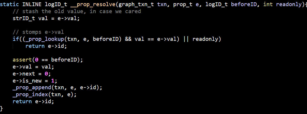
Setting a property ends up calling _prop_resolve() which looks like this:

image

Again, very similar to what we have seen before. This is a good thing. Predictability in a code base is a very nice property (pun intended).

Properties are indexes on:

  • parent, key –> id

In other words, you can lookup the properties of a node (or an edge) based on its parent or type. Interestingly enough, it isn’t indexing the value of a property. I would expect to have an index on (key, value –> id), which would allow for richer queries. On the other hand, I guess they do most / all of their queries on the type/val pair as the source.

With this, I feel like I have a good grasp on what is going on in LemonGraph in terms of the on disk data structure. In the next post, I’m going to try to figure out how it is handling queries.

time to read 7 min | 1294 words

A few months ago the NSA released LemonGraph, a graph database based on LMDB. This weekend I took the time to explore the codebase. As usual, I’m going to be reading the code in lexical order, and mostly trying to figure out where things are happening and what the code is doing.

I started to read the Python code, but it immediately called to native C code:

image

Looking at the lemongraph.h file, I see a lot of quite interesting methods. This looks like the heart of LemonGraph is implemented in C, while the higher level Python code is orchestrating things. Not sure if this is a fair statement, but I’m going to be reading some C code now.

image

The first interesting thing in the C code is that LemonGraph actually wrapped LMDB with their own interface. From db.c, we have:

image

The MDB_xyz flags are defined by LMDB, DB_xyz are defined by LemonGraph. I assume that this was done to hedge their bets with regards to the underlying storage engine. From my own experience, any such attempt is usually doomed to failure. It isn’t the compilation errors that will kill you but the different behavior that you are coupled to that matters. A lot of the code there is basically forwarding directly to LMDB, but there is actual behavior implemented in db.c. In particular, they seem to have a lot of logic around managing remapping of LMDB (which is fixed size and requires reopening to change).

The lemongraph.c file is about 1,750 lines in size. I skimmed it a bit, but let’s get to the interesting bits. I tried to check where it is creating a new node and follow the code from there, but I got lost. So I started with the docs and looked at this code:

image

As a reminder, I’m reading this code in a text editor, not running it, so I’m somewhat limited by what I can discover. This Python code is strange, because it is doing creation by omission. In other words, if you already had a a node with “foo:bar” there, it would return it. Otherwise, a new node is created. Not my cup of tea, but make sense for a Python interface.

Let’s dig deeper into how this is built, shall we? This call ends up here:

image

This then calls to:

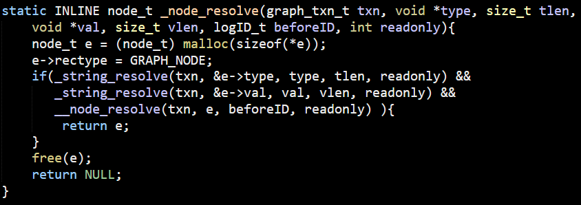
image

I want to stop everything for a moment and look at the first line of this code. It calls malloc, and it does this in a pretty strange manner. Note that it looks likes it dereferences the variable before it has been initialized. This isn’t what is actually going on.

The sizeof operator is a compile time feature. And this relies on this code:

image

In C, structs are referred to as “struct STRUCT_NAME” and are typically typedef to themselves to make things easier. In this codebase, there is “struct node_t” and “node_t”, which is a pointer to the struct. I find this very confusing, to be honest.

At any rate, back to _node_resolve method. You can see something pretty interesting here. we have the _string_resolve method. What is it doing there? This just forward the call to __resolve_blob, which is really interesting.

It is a bit long, and you can read it at your leisure here. The signature is here:

image

Basically, it uses a feature of LMDB that allow to store multiple values for a key. I started describing what this is doing, but then I realized that this is crazy. Sample code would be much easier. Here is the essence of this method:

As you can see, the idea is that LemonGraph maintains an internal string index, allowing it to turn any existing string into a numeric id. Going back to the _node_resolve() method, you can see that the _string_resolve method is used to get a unique id for both the type and val parameters. This is then sent to the __node_resolve() method.

As an aside, I’m loving the fact that you can figure out the call graph for methods based on the number of underscores prefixed to the name. No underscore, public method. Single underscore, private method used internally. Two underscores, hidden method, used sparingly. At three underscores, I could tell you what it means, but given that this is NSA’s codebase, I’ll have to kill you afterward.

image

This is a nice method. We first do a lookup, and if it isn’t there, we’ll append a new node. I’m going to look at the _node_append() method first, because it will likely make looking at the _node_lookup() method easier.

image

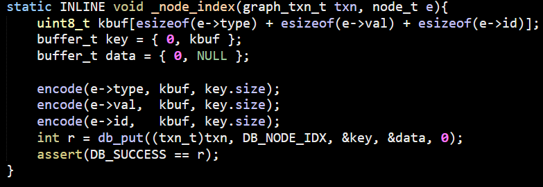
The encode() method uses length prefixed ints to encode int64 values in fewer bytes. I’m not sure why they chose this format over variant size int. That would save at least one byte in almost all cases. The end result of this method is that we pass the dbuf buffer to the _log_append() method with the (next, type, val) values encoded in it. I’m not sure what next is at this point, but I know that in the case we have here, this is meant to be 0, so we can probably ignore it for now. The _log_append() method simply append the buffer to a tree and returns a sequential id, nothing more. Going back up a bit, the _node_index() is now called, which looks like this:

image

This is basically is just adding the value to the log and creating an index to search by (type,val) – giving the id. This just make me that much more interested in the next. I’m pretty sure that this is required for a feature they call historical views, which likely means that they never actually do deletes, just markers. This is a nice feature if you want to effectively go back in time, or maybe compare current and past events.

On the one hand, this limits the usability of the graph, because your data set will only grow. On the other hand, not having to worry about deletes is so much easier.

Now we can go and figure out what is going on with the _node_lookup() method.

image

You can see that this is using the same DB_NODE_IDX from the _node_index() method. So basically this is doing the reverse of the past few methods. This will lookup the index, then fetch the relevant log id for this.

This is enough for now, I have a good grasp of the basic underlying data structures. I’m pretty sure that now that I know how nodes works, I can quickly check how edges and properties work as well. Hopefully, next post will be able to talk about the graph operations directly, but I might run into other interesting bits first.

FUTURE POSTS

No future posts left, oh my!

RECENT SERIES

  1. Challenge (75):
    01 Jul 2024 - Efficient snapshotable state
  2. Recording (14):
    19 Jun 2024 - Building a Database Engine in C# & .NET
  3. re (33):
    28 May 2024 - Secure Drop protocol
  4. Meta Blog (2):
    23 Jan 2024 - I'm a JS Developer now
  5. Production Postmortem (51):
    12 Dec 2023 - The Spawn of Denial of Service
View all series

Syndication

Main feed Feed Stats
Comments feed   Comments Feed Stats
}