I’m currently working on a pretty deep optimization cycle in how RavenDB and Voron (its storage engine) handle I/O. The idea is to be able to squeeze more performance out of the system by being able to utilize a lot of moving pieces at once (parallelizing compute, durable I/O, async I/O, etc.).

At the end of the day, however, it all must reside on disk, of course. That means that I’m essentially seeing how close I can dance to the edge of the capabilities of the system. For example, let’s consider AWS GP3 drives. They offer 3K IOPS and 125MB/sec on the basic plan.

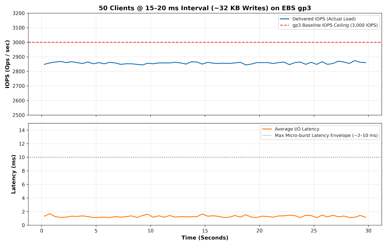
We have 50 clients, each generating a request every 15 - 20 ms and writing ~32KB each. This is the kind of load that they’ll generate on the system. Here is what this looks like:

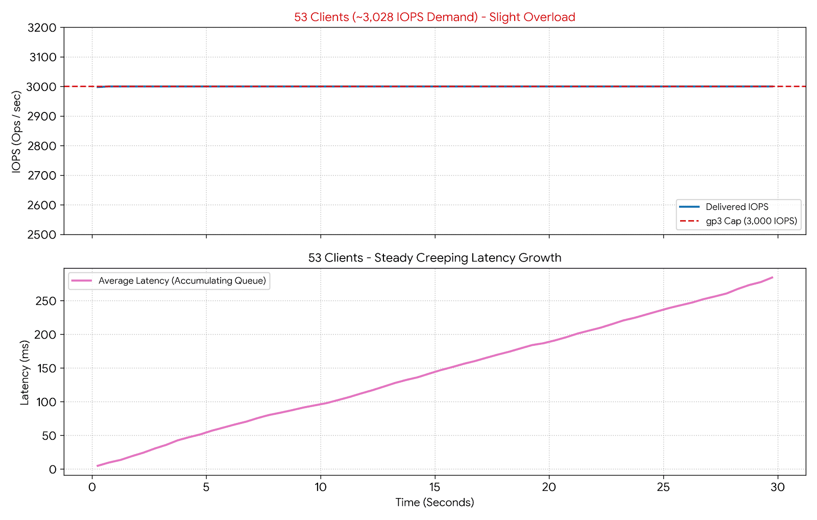
Now, let’s add just 3 additional clients to the mix, add just enough to hit the limit (not even grossly exceed it!). Here is what this looks like:

Note that in very short order, we moved very quickly from < 2ms to > 250 ms. That is the kind of dangerous tipping point that causes the system to just fall over and die.

As a database engine builder, I have to be really conscious about those details, since it is better for us to start rejecting or slowing requests before we saturate the disk like that. When this happens, you often can end up with a system that is simply unable to perform any I/O.

When that happens, you start using more memory (and buffers). When you run out of memory, the OS will decide to try to swap to disk. But the disk is busy. I/O starvation like that can turn into “the entire machine just locked up and doesn’t respond to anything” in very short order.

I have shown you AWS GP3 for a reason; it has consistent behavior. But there are other models. AWS GP2, Azure’s Premium SSD v1, and GCP’s Standard PD all have a different mechanism.

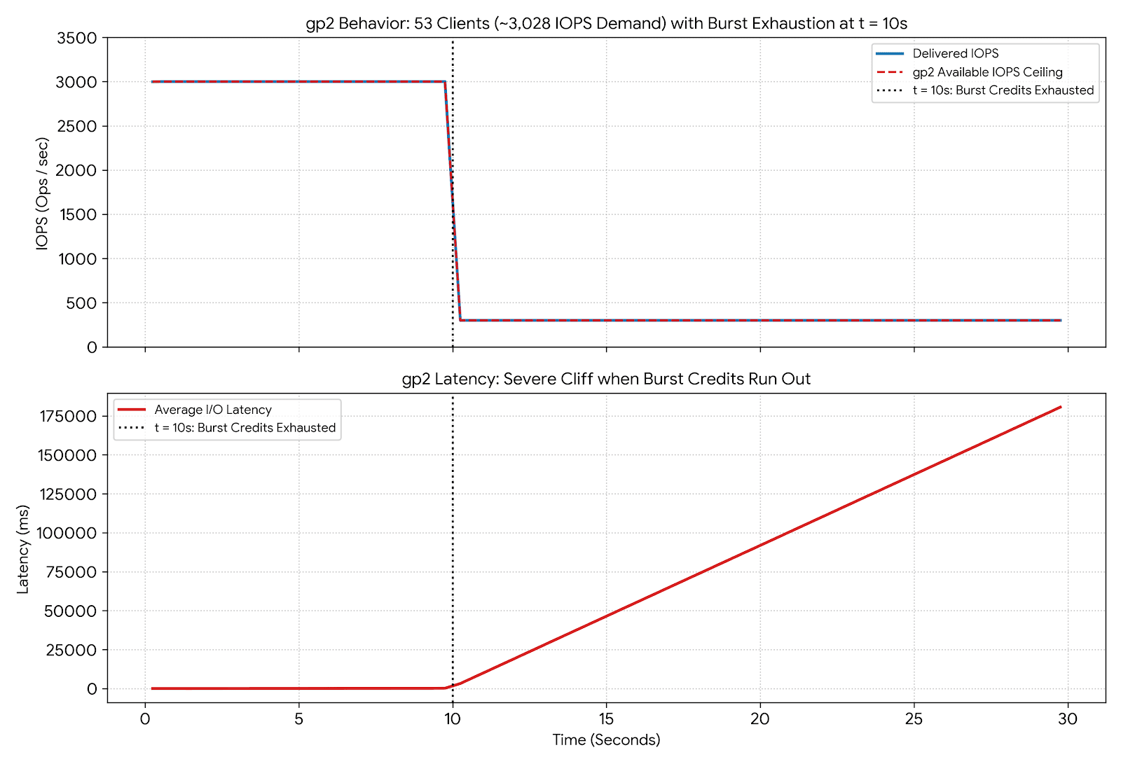
You get burstable I/O - if you need to copy a large file, for example, the system will let you exceed those limits (for a while). You get a certain allowance that allows you to smooth over jumps in usage. That can be very nice, until you realize that this is what this does to the system:

I strongly dislike those sorts of disks, because there is very little that you can do to actually properly prepare for these scenarios. At one moment, you are running smoothly, and suddenly all your I/O is yanked out of your hands. You don’t have time to apply back pressure, for example. It’s like going for a jog and at the 800m line you are wearing lead shoes.

As they say, as a result: hilarity ensues.

All of this exposition is to discuss the details of what I’m trying to do. The work we are doing is to try to make the most of the hardware capabilities we have, and at the same time, be able to apply back pressure on our clients so we can properly perform at high scale.

I’m doing this work with Claude Fable 5. At the time of this writing, this is one of the top frontier models. I find it quite an interesting experience, to be honest. It is like working with an idiot savant, with an emphasis on both parts at once.

It can be incredibly capable of wedging itself into weird shapes. The reason for this post is that I’m currently waiting for a benchmark run to complete and contemplating this statement that it based a whole design on:

bandwidth = maximum size/duration ever observed (a flood cannot make a single write exceed the device's real throughput, so congestion can't inflate this either).

As you can see, this assumption (which was “load bearing” for the entire design) is quite wrong. It is also the sort of thing that caused me to have a jump scare moment when I saw that. No, we do not make these sorts of assumptions here. Don’t ask me why; I got the scars from that.

The interesting part of this assumption is that it is entirely reasonable to make. If I heard that statement from a developer, I would correct that, but it would make sense why they think that.

For a frontier model (that is currently busy doing this exact performance work, I should add), that was surprising. It showed how a small assumption can generate a pretty bad result. To be fair, I had my own similar scenario (which took ~10 years to fix).

I can say that you can expect some nice goodies out of this work.

A while ago, MongoDB purchased VoyageAI for 220 million dollars. Since then, they have released a couple of dedicated embedding models. For example, you can read their blog post on voyage-context-4.

The key premise in those sorts of models is that you can feed the model text of any size, and it will automatically handle generating embedding vectors, smart chunking, providing context, etc.

I ran into this recently and was curious to see how this can work. In particular, since RavenDB handles both embedding generation and vector search, I decided to do a full evaluation of MongoDB’s way of chunking. MongoDB built their own model to achieve this, but RavenDB’s approach to embedding generation is to rely on any embedding model you prefer to use.

Before we get into the full details, let’s talk for a second about what the point of contextual embedding is, so we are all on the same page.

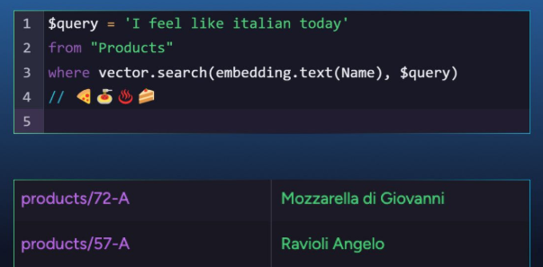
Embedding models take your data and translate it into a multidimensional mathematical space based on its meaning. Similar items will be located near one another in this multidimensional space, and we can take advantage of that using vector search. That is why you can find Mozzarella & Ravioli if you want Italian food today, as in this example:

The problem is that all embedding models have a context limit. There is only so much text that you can push into the model before it will give up on you. If you want to search through a much bigger piece of text using semantic search, you need a different approach.

The industry standard approach to handling this is via chunking. In other words, you take a long piece of text, split it into separate parts called chunks, and generate an embedding for each one separately.

The easiest way to think about this is that you have a long document, and you generate a separate embedding vector for each page of text independently. Instead of having to digest a whole article, you feed a bounded chunk (page) to the model to generate an embedding vector.

Chunking is a neat trick, but it leads to its own set of problems. Assuming we have a large document that talks about new features in RavenDB, with a particular page that expounds on the details of “the database’s ACID guarantees". What would the embedding vector for that page look like?

If we just chunk the data naively, we’ll get a vector that is related to the generic concept of ACID in databases. The chunking approach loses the context of the data; it doesn’t understand that the database in question is RavenDB.

Contextual embedding allows you to bake a global perspective directly into every chunk’s embedding. In other words, the embedding for that page would know that the database that is being talked about is RavenDB.

If you are dealing with large texts and want to have high-quality search, contextual embedding is a feature you want. I guess that explains why MongoDB paid 220 million dollars for Voyage AI.

Sadly, I left that sum of money in my other pants, so RavenDB’s strategy for dealing with this scenario is quite different. We planfor models to become a commodity, so there is little benefit in trying to produce your own models at this point in time.

Instead, RavenDB takes the approach of working with all off-the-shelf models. That means that we are far more flexible, using the latest state-of-the-art models, instead of having to keep chasing them. But only some models support contextual embedding…

Luckily, we figured out that we can add this feature from RavenDB’s side, without needing to develop a custom embedding model for this. The technical announcement about it is here, with all the details. But the gist of it is that RavenDB allows you to attach context to the value you send for embedding.

The scenario below shows an example of storing litigation files using RavenDB and enabling proper semantic search over large amounts of data:

const tokenCount = 2048;
const overlap = 128;


const chunk = (field) => text.splitParagraphs(field, tokenCount, overlap);


embeddings.generate({
  FullDetails: chunk(this.FullDetails),
  CaseSummary: chunk(this.ExtractedSummary),
  PartiesInvolved: chunk(this.MetadataParties),
  Precedents: chunk(this.CitedAuthorities),
  RatioDecidendi: chunk(this.CoreLegalRules),
  ObiterDicta: chunk(this.DissentingArguments)
})
.withContextPrefix(this.Headline);

You can see that we generate embeddings for quite a few fields. For all of them, we use a chunking strategy of 2K tokens with an overlap of 128 tokens. Note the last line that adds a withContextPrefix call, where we add the Headline as part of the context for the data we’ll be embedding.

This additional context gives the embedding model enough information to contextualize the information we give it. The nice thing about this feature in RavenDB is that we don’t need to have any special support from the model. Everything is handled directly by RavenDB. That includes chunking, caching, adding the context, etc.

What to do when I don’t have pre-existing context to add?

If you have a title for an article, or a summary already written for you, that is great. But what happens when no such thing exists? You can also use GenAI tasks in RavenDB to process the data and get a proper summary (and then generate the embedding with that summary to have better queries).

I took the context prefix feature for a spin with a bunch of well-known datasets in the field of embedding and retrieval. We are using nDCG@10 — normalized Discounted Cumulative Gain at rank 10, the standard retrieval-quality metric on the public BEIR, LoCoV1, and LongEmbed benchmarks.

The underlying embedding model we use is OpenAI’s text-embedding-3-small, and we use exact() vector search in RavenDB, since we are testing purely the embedding output.

Adding context to chunked documents

For the following benchmarks, we defined two embedding tasks. One that would simply generate chunked embeddings from the raw text (with 256 tokens per chunk), and another with additional context taken from the document’s title.

embeddings.generate({ 
    ContentEmbedding: text.split(this.Content, 256)
        .withContextPrefix(this.Title) 
});

TREC-COVID        +9.2

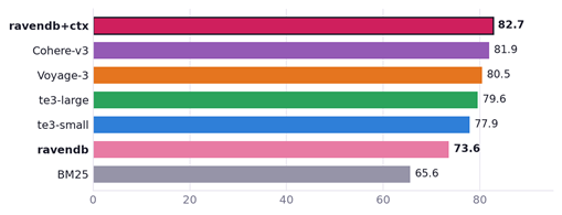
COVID-19 literature comprising ~129K near-identical CORD-19 papers with short, keyword-like queries. The abstracts all look alike, so the paper’s title is the single most discriminating signal. You can see that this approach is able to provide better results than any of the other options.

Fair benchmarks are hard (we made it harder for us)

In the following benchmarks, the ravendb and ravendb+ctx entries are the only ones that are actually using chunking. In other words, all the other alternatives are getting the full document to work on. And indeed, you can see that the ravendb entry (which does native chunking) isn’t doing that well in this benchmark. With the added context, it reaches the top.

Chunking at 256 tokens was used because it is a reasonable chunk size (about two paragraphs of text), and at that size, you may lose the context of the overall document. This allows us to showcase how effective the additional context technique is. That is also quite useful for additional focus. Embedding quality degrades with the length of the text, so shorter chunks embed their concepts much more faithfully.

NFCorpus        +2.8

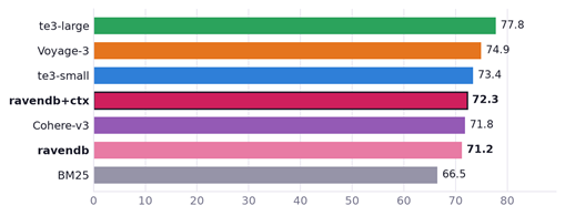
Consumer-health and nutrition queries matched against PubMed documents. Titles name the medical topic (such as a condition or a nutrient), which disambiguates heavily overlapping biomedical text; the prefix lifts us past published text-embedding-3-small results. In fact, only text-embedding-3-large is able to do better than us here (see below for benchmark results showcasing RavenDB’s approach with text-embedding-3-large).

SciFact        +1.1

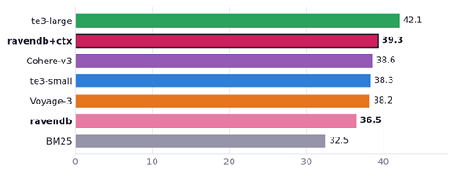
Scientific-claim verification against research-paper abstracts. The title names the paper’s specific finding, nudging near-duplicate abstracts apart, but the abstract is already on-topic. The gain is modest, and we land within a point of the published te3-small score.

As you can see, in this case ravendb+ctx is doing better than ravendb. However, I wouldn’t say that it is doing well. The chief problem is that chunking to such a small size really hurts us, and just using the full document is better.

Testing additional context with text-embedding-3-large

We intentionally test this approach with a modest model (text-embedding-3-small that has ~100M - 300M parameters). Does this approach scale when we use a bigger model? The text-embedding-3-large model is estimated to be in the 1B - 2B parameter range. How does it behave when we use the same technique?

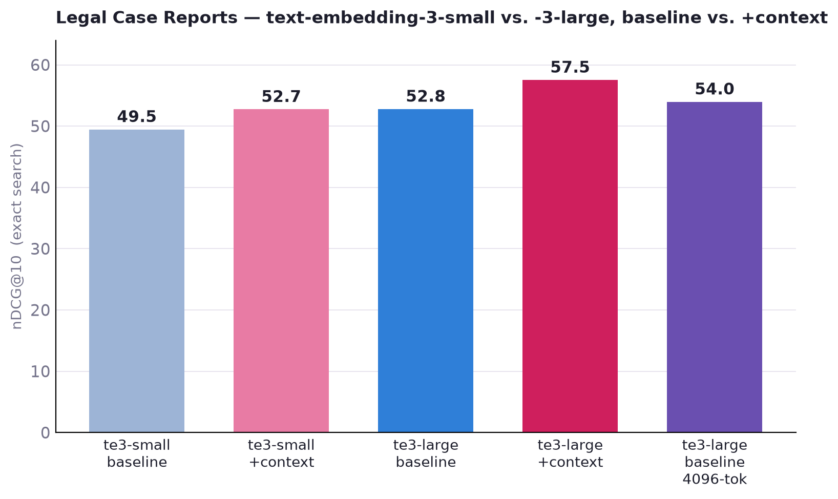
In the graph below, we are testing the Legal Case Reports dataset, which has a lot of large documents (some with > 100K tokens and many over the 8K token limit).

We tested the quality of the results with chunking of 256 and 4096 tokens.

You can see in the graph that text-embedding-3-large is indeed better than text-embedding-3-small. There is a +3.3 difference between the baseline numbers of both models.

With the context option, however, text-embedding-3-small is almost as good as text-embedding-3-large! And with context, text-embedding-3-large ismuch better.

We also tested text-embedding-3-large with a much larger chunk size of 4K, which should give it more context to draw on (but also dilutes that contextt). Even so, it wasn’t able to beat the additional context (with a much smaller chunk size).

Dealing with large documents

The previous datasets we dealt with all had documents that fit nicely within an embedding model context window. Now we are going to deal with much longer documents (5K–470K tokens each). To make things more interesting, these have no natural title to anchor a chunk.

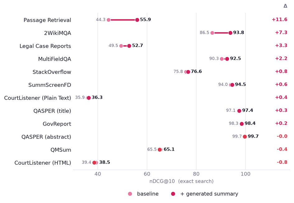
To handle this, we use another RavenDB AI feature, GenAI Tasks, which reads the first 16K of the document and generates a short summary for it. We then use that summary as the additional context for the chunking.

Without further ado, here are our results:

Those datasets were taken from the LoCoV1 and LongEmbed datasets. They are quite large and are usually used to explicitly test handling very large documents.

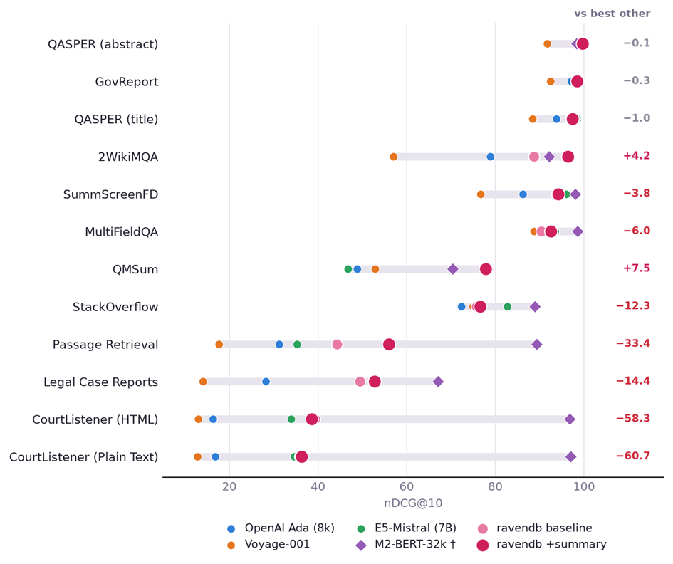
You can see that this technique shows a measurable impact on most (but not all) of the datasets we have tested. It gets more interesting when you compare it head to head with the actual results of the LoCoV1 and LongEmbed papers.

The results we are showing here show us being worse on almost every level, which would typically be a Bad Thing. In this case, we are comparing RavenDB using an off-the-shelf embedding model (with chunking!) versus dedicated top-tier embedding models that process the whole document.

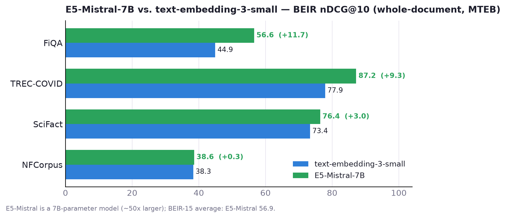
Across almost every task RavenDB is able to exceed the results of OpenAI Ada, Voyage-001, and E5-Mistral-7B.  Let’s take E5-Mistral-7B as a good example. It is a 7B parameters, while text-embedding-3-small has only 100M - 300M parameters, making it about 50 times smaller.

The following graph was extracted from E5-Mistral paper (arXiv 2401.00368), Table 17 and should give you a pretty good idea about how the two models compare:

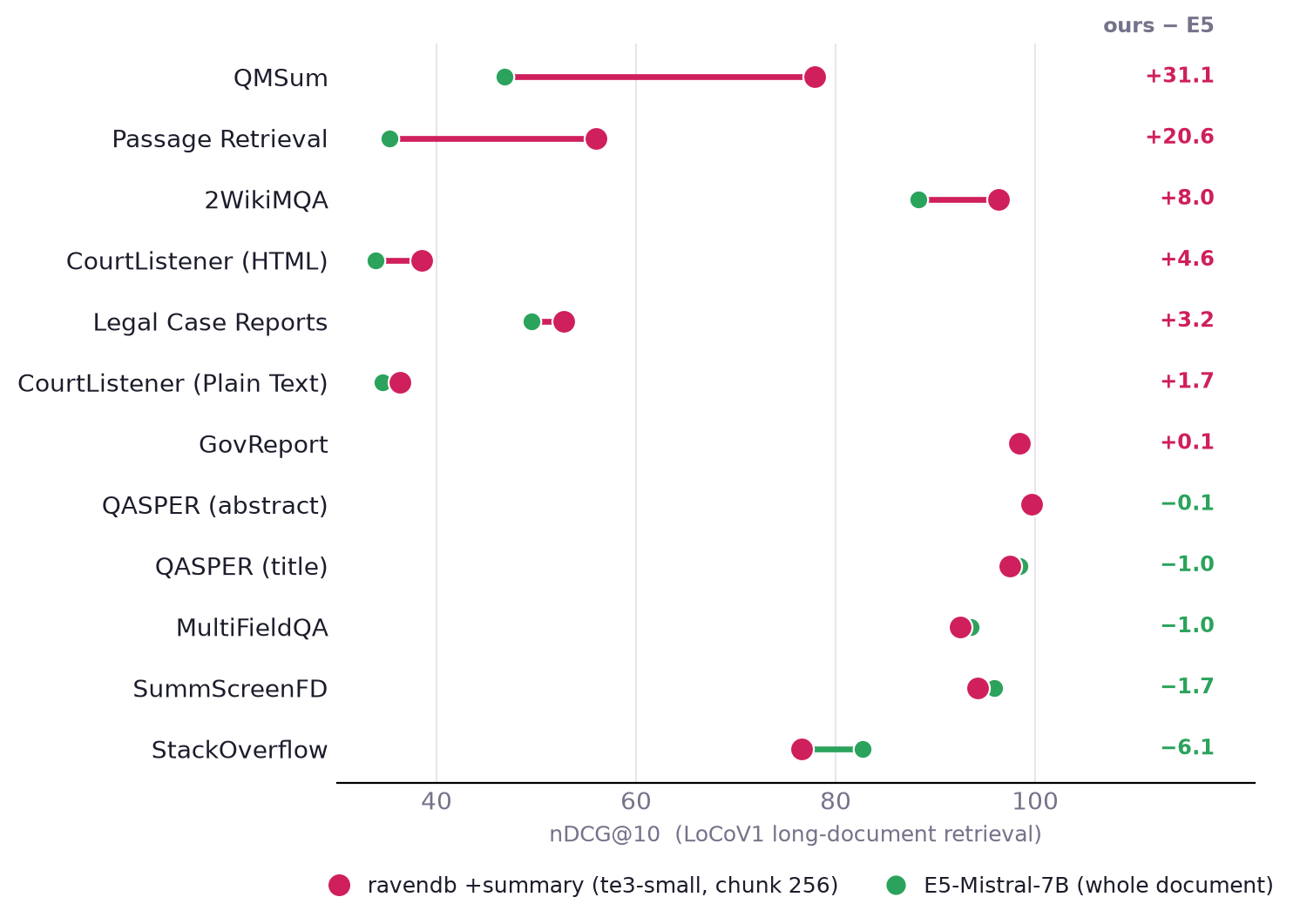
On the other hand, when we use the same text-embedding-3-small and our context prefix approach, we get the following results:

The most interesting thing about this graph is what this means. There is a very clear divide between the datasets where E5-Mistral-7B is leading and those where RavenDB’s approach leads (with a much smaller model).

The whole-document 7B model dilutes long text into one vector; our approach keeps focused chunks and restores document context via the summary. In the datasets composed of short documents, Mistral wins handily (it's a 7B model, ~50× bigger).

On long documents, RavenDB’s approach flips that by large margins when the answer is spread across the document (QMSum, passage retrieval, multi-hop QA). On long documents the chunk+context prefix strategy buys much more than raw model size does.

The 7B model reads the whole document into one vector and gets diluted; the small model retrieves a focused chunk and gets its document context back from the summary.

Summary

RavenDB’s context prefix feature shows how a different architecture can get you better results and higher efficiency. RavenDB’s approach allows us to go head to head with dedicated models and still come out ahead when dealing with large documents and complex tasks.

It also works on any model. I used text-embedding-3-small specifically because it is a baseline model, not a top-tier one. The fact that this is model-agnostic means that you can tune your approach based on your dataset and your requirements. When a new (and better) model comes by, you can just move to it and still reap the benefits.

This approach won’t cost you 220,000,000 USD. I just checked, and producing this blog post cost us about $110 (most of that by generating summaries for the large documents, to be honest). Only $22 of that was spent on the actual embedding.

Pair a DGX or Mac Studio in a cupboard with Gemma 4 (another great 7B embedding model) and RavenDB’s context prefix mode. You get top-tier results for a one-time ~$4,000 USD hardware investment, with no monthly bills.

* You can find the code to reproduce the findings in this post in the following GitHub repository.